


-
合成孔径激光雷达(SAL)是激光技术与合成孔径技术的结合,相比于微波雷达(SAR)具有更高的分辨率。近十几年来,SAL发展较快,国内外分别实现了室内[1-6]和室外机载SAL[7-9]成像实验。由于空间中没有大气湍流和大气衰减等问题,激光在空间中传输的衰减较小,因此,相对于地基和机载SAL,天基SAL更有优势[10]。且卫星具有预警、侦查、中继和通信等功能,具有特殊的军事及民用价值,若能对他国卫星进行高分辨率成像,便可获取他国卫星的结构、尺寸和卫星承担的任务等信息。同时,若我国卫星发生故障,对故障卫星的高分辨率成像也可诊断出故障原因[11]。因此,天基SAL高分辨率成像具有重要的应用价值,应用前景广泛。
由于天基SAL的实验成本高,因此目前这方面的实验还不够成熟。为对太空进行探测、识别和鉴定威胁行为,并增强太空感知,美国空军研究实验室在2018年4月发射了EAGLE实验卫星,在地球同步轨道(GEO)上进行天基SAL对其他GEO目标成像的技术验证,但并没有明确报道[12],而国内的研究目前都处于理论阶段。
2012年,李今明等人初步设计了一种适于对静止轨道卫星成像的载星轨道,并提出两星相距最近时刻是成像的最佳时期,可采用径向速度门限来判定目标是否已进入最佳成像时机[13]。2013年,阮航等人利用天基逆合成孔径激光雷达(ISAL)对静止轨道目标成像,认为逆行轨道上的卫星对静止轨道卫星成像时,具有重访率高、短时间成像的优点[11]。2016年,李飞等人建立了对非合作目标进行高分辨率成像的天基SAL成像模型,并对地球静止轨道上的目标进行了系统设计[14]。2019年,李丹阳等人提出在两卫星交会点附近连续长时间观测的思路,并以匀速直线运动为近似观测模型,给出了天基SAL成像流程[15]。本文将在以上研究的基础上,通过成像参数分析,进一步验证天基中高低轨卫星间SAL成像的可行性。
根据卫星运行轨道的高度,将卫星分为低轨卫星(小于1000 km)、中轨卫星(1000~20 000 km)和高轨卫星(大于20 000 km)三种。首先,建立天基SAL成像模型,对天基SAL的合成孔径时间和成像分辨率进行理论推导。其次,采用二体运动轨道外推法,建立激光雷达搭载卫星和成像卫星的轨道模型,并根据雷达天线波束宽度的限制,计算激光雷达的收发天线方向图,利用目标增益曲线的3 dB宽度,计算SAL最大合成孔径时间。最后,通过仿真,建立中高低轨卫星间的六种应用方式,得出不同应用方式下的最大合成孔径时间以及最大合成孔径时间内,两卫星间的多普勒带宽、相对距离、相对速度和相对加速度等参数,进而验证天基中高低轨卫星间SAL成像的可行性,并为天基SAL成像算法的研究奠定基础。
-
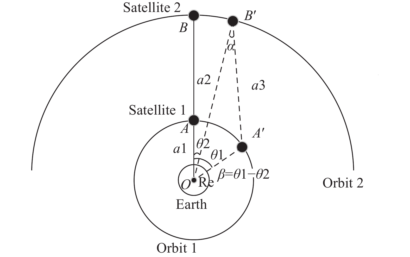
根据卫星运行轨道的高度,可将卫星分为低轨卫星、中轨卫星和高轨卫星三种。天基SAL成像几何示意图如图1所示。
假设卫星1的和卫星2相对地心的轨道高度分别为a1和a2,地球半径Re为6 378.14 km。根据轨道高度,可确定卫星运行周期为:
$${T_{\rm s}} = 2\pi \sqrt {\frac{{{a^3}}}{\text{μ}}} $$ (1) 式中:
${\text{μ}} = {\rm{3}}{\rm{.986\;004\;7e14}}\;{{{\rm m^3}}/{{\rm s^2}}}$ 为开普勒常数;$a$ 为卫星轨道半长轴。根据卫星运行周期,可确定卫星相对地心的转动角速度为:$$\omega = \frac{{2\pi }}{{{T_{\rm s}}}} = \sqrt {\frac{\text{μ}}{{{a^3}}}} $$ (2) 由图1可知,初始时刻,卫星1和卫星2与地心连线重合,假设SAL成像的合成孔径时间为
$\Delta t$ ,经过很短的时间$\Delta t$ 后,卫星1从位置A转动到A'处,卫星2从位置B转动到B'处。假设$\Delta t$ 时间内卫星1和卫星2相对地心的转动角度分别为$\theta 1$ 和$\theta 2$ ,则两卫星相对地心转动的角度差为:
图 1 天基合成孔径激光雷达成像几何示意图
Figure 1. Geometric diagram of spaceborne SAL imaging
$$\beta = \theta 1 - \theta 2 = \Delta t\left| {\omega 1 \pm \omega 2} \right|$$ (3) 式中:
$\omega 1$ 和$\omega 2$ 分别为卫星1和卫星2相对地心的转动角速度,$\omega 1 - \omega 2$ 表示两卫星的运动方向相同,$\omega 1 + $ $ \omega 2$ 表示两卫星的运动方向相反。由图1可知,在合成孔径时间
$\Delta t$ 内,两卫星间的相干积累角为$\alpha $ 。在三角形OA'B'中,有关系式:$$\frac{{a3}}{{\sin \beta }} = \frac{{a2}}{{\sin \left( {\pi - \beta - \alpha } \right)}} = \frac{{a1}}{{\sin \alpha }}$$ (4) -
SAL成像是一种高分辨率成像方式,其图像分辨率用距离向分辨率和方位向分辨率描述。其中,距离向分辨率
${\rho _{\rm r}}$ 由发射信号带宽$B$ 决定,距离向分辨率公式为:$${\rho _{\rm r}} = 1.2\frac{C}{{2B}}$$ (5) 式中:
$C$ 为光速。由上式可知,距离向高分辨率可以通过发射大时宽带宽信号实现。当距离向分辨率为5 cm时,发射信号带宽可设置为3.6 GHz。方位向分辨率
${\rho _{\rm a}}$ 由雷达与目标星的相干积累角$\alpha $ 决定,方位向分辨率公式为:$${\rho _{\rm a}} = \frac{\lambda }{{2\alpha }}$$ (6) 式中:
$\lambda $ 为发射信号波长。由上式可知,方位向分辨率的大小由$\alpha $ 决定。由于天线波束宽度和两卫星间相对位置关系的限制,目标卫星不可能一直被激光雷达信号照射到,而相干积累角$\alpha $ 由目标卫星被照射的时间(即相干积累时间$\Delta t$ )决定。因此,本文主要通过分析星对星SAL成像的相干积累时间,说明星对星SAL成像的可行性。为达到方位向分辨率的要求,需要两卫星间的相干积累角满足条件:
$$\alpha = \frac{\lambda }{{2{\rho _{\rm a}}}}$$ (7) 式中:
$\lambda $ 为发射激光波长;${\rho _{\rm a}}$ 为方位向分辨率。根据公式(3)、(4)、(7)可知,两卫星进行SAL成像的相干积累时间$\Delta t$ 为:$$ \begin{split} \Delta t =& \dfrac{\beta }{{\left| {\omega 1 \pm \omega 2} \right|}} = \dfrac{1}{{\left| {\sqrt {\dfrac{\mu }{{a{1^3}}}} \pm \sqrt {\dfrac{\mu }{{a{2^3}}}} } \right|}} \times \\ &\left( {{\rm arc}\sin \left( {\dfrac{{a2}}{{a1}}\sin \left( {\dfrac{\lambda }{{2{\rho _{\rm a}}}}} \right)} \right) - \frac{\lambda }{{2{\rho _{\rm a}}}}} \right) \\ \end{split} $$ (8) 由上式可知,两卫星间的相干积累时间与两卫星的运行方向有关,与轨道高度、分辨率和波长有关。
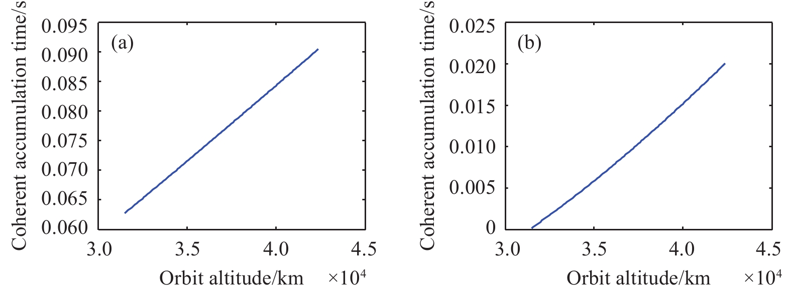
若用1 064 nm激光,实现5 cm分辨率成像。利用轨道高度为700 km的低轨卫星,与800~36 000 km轨道高度的卫星做SAL成像;利用轨道高度为15 000 km的中轨卫星,与15 100~36 000 km轨道高度上的卫星做SAL成像;利用轨道高度为25 000 km的高轨卫星,与25100 ~36 000 km轨道高度上的卫星做SAL成像,设置相同和相反的运行方向,观察不同轨道高度和不同运行方向时两卫星的相干积累时间曲线。
图2~4中横坐标表示卫星轨道高度,纵坐标表示相干积累时间,根据曲线变化趋势可知,两卫星相距越远,所需的相干积累时间越长;两卫星运行方向相反时所需的相干积累时间较两卫星运行方向相同时短;由于700 km低轨卫星与36000 km高轨卫星的相干积累时间小于0.06 s,15000 km低轨卫星与36000 km高轨卫星的相干积累时间小于0.09 s,25000 km高轨卫星与36000 km高轨卫星的相干积累时间小于0.095 s,说明中高低轨卫星间在较短的时间内就可以实现SAL成像。

图 2 700 km高度轨道卫星的相干积累时间曲线。(a)两卫星运行方向相同;(b)两卫星运行方向相反
Figure 2. Coherent accumulation time curve of 700 km high orbit satellite. (a) Two satellites run in the same direction; (b) Two satellites run in opposite directions
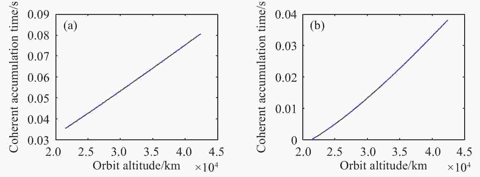
图 3 15000 km高度轨道卫星的相干积累时间曲线。(a)两卫星运行方向相同;(b)两卫星运行方向相反
Figure 3. Coherent accumulation time curve of 15000 km high orbit satellite. (a) Two satellites run in the same direction; (b) Two satellites run in opposite directions
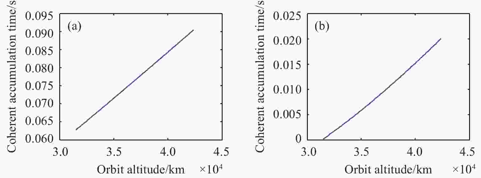
图 4 25000 km高度轨道卫星的相干积累时间曲线。(a)两卫星运行方向相同;(b)两卫星运行方向相反
Figure 4. Coherent accumulation time curve of 25000 km high orbit satellite. (a) Two satellites run in the same direction; (b) Two satellites run in opposite directions
-
方位向相干积累过程中,多普勒频率为[16]:
$$ \begin{split} {f_{\rm d}} =& \dfrac{{2\left| {{w_1} - {w_2}} \right|}}{\lambda }r = \\ &\dfrac{{2\left| {\sqrt {\dfrac{\mu }{{a{1^3}}}} \pm \sqrt {\dfrac{\mu }{{a{2^3}}}} } \right|}}{\lambda }r \\ \end{split} $$ (9) 式中:
${w_1}$ 和${w_2}$ 分别为卫星1和卫星2的线速度;$r$ 为目标长度在转台模型横轴上的投影。则整个合成孔径期间内,多普勒带宽为:$$\Delta {f_{\rm d}} = \frac{{2\left| {\sqrt {\dfrac{\mu }{{a{1^3}}}} \pm \sqrt {\dfrac{\mu }{{a{2^3}}}} } \right|}}{\lambda }L$$ (10) 式中:
$L$ 为目标星的长度,为避免方位向模糊,脉冲重复频率PRF应大于$\Delta {f_{\rm d}}$ 。 -
轨道六根数包括轨道半长轴
$a$ 、轨道倾角$i$ 、升交点赤经$\Omega $ 、近地点幅角$\omega $ 、偏心率$e$ 、真近点角$f$ 。根据轨道六根数,以地心为坐标原点,建立如图5所示的地心轨道坐标系。
图 5 地心轨道坐标系示意图
Figure 5. Schematic diagram of geocentric orbit coordinate system
卫星过近地点时
$t = 0$ ,$f$ 为真近点角,$E$ 为偏近点角,$r$ 为卫星相对地心瞬时位移。对于理想的二体运动模型,根据上图的几何关系,得到卫星到地心的距离$r$ 和轨道时间$t$ 的函数,即为不同时刻卫星相对地心的位置坐标[17]。 -
由于天线波束宽度和两卫星间相对位置关系的限制,目标不可能一直被激光信号照射到,因此,需要对波束照射时间进行计算,观察激光雷达对目标星的照射时间是否大于相干积累时间
$\Delta t$ 。首先,根据天线波束宽度,计算卫星收发天线的二维方向图,二维方向图表示天线波束范围内不同方位角和俯仰角上的增益,可用二维sinc函数表示。其次,以SAL搭载卫星的质心为原点,建立卫星天线坐标系,计算目标卫星相对搭载卫星的增益曲线。最后,根据目标卫星增益曲线的3 dB宽度,计算目标卫星可以被照射的时间,与
$\Delta t$ 对比,若目标卫星被照射时间大于$\Delta t$ ,说明目标卫星可以满足成像分辨率的要求,反之,则说明目标卫星不能满足成像分辨率的要求。假设激光雷达天线在方位向和俯仰向的波束宽度分别为
${\gamma _{\rm a}}$ 和${\gamma _{\rm p}}$ 。利用衍射光学系统[12],根据相控阵原理[18],可将天线近似成大小为${\lambda /{{\gamma _{\rm a}}}} \times {\lambda /{{\gamma _{\rm p}}}}$ 的阵列天线,因此可根据增益公式分别计算方位向和俯仰向的一维方向图:$$ \begin{split} {G_{\rm a}} = & \displaystyle\sum\limits_{m = 0}^{M - 1} {\exp \left(j\dfrac{{2\pi }}{\lambda }md\sin {\phi _{\rm a}}\right)} , \\ &{\phi _{\rm a}} \in \left[ { - {{{\gamma _{\rm a}}} / 2},{{{\gamma _{\rm a}}} / 2}} \right] \\ \end{split} $$ (11) $$ \begin{split} {G_{\rm r}} = & \displaystyle\sum\limits_{n = 0}^{N - 1} {\exp \left(j\dfrac{{2\pi }}{\lambda }nd\sin {\phi _{\rm r}}\right)} \\ &{\phi _{\rm r}} \in \left[ { - {{{\gamma _{\rm r}}}/2},{{{\gamma _{\rm r}}}/2}} \right] \\ \end{split} $$ (12) 式中:
$d = {\lambda/2}$ ;$N = ceil\left( {{\lambda /{{{{\gamma _a}}/d}}}} \right)$ ;$M = ceil\left( {{\lambda /{{{{\gamma _{\rm p}}}/ d}}}} \right)$ ,$ceil$ 表示向上取整。则二维天线方向图可表示为:$$G = {G_{\rm a}}G_{\rm r}^{\rm T}$$ (13) 图6为天基合成孔径激光雷达发射天线一维和二维方向图,由于俯仰向的一维方向图和方位向的一维方向图相同,这里只给出了方位向的一维方向图。
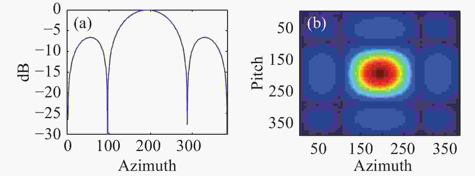
图 6 天线方向图。(a)方位向一维天线方向图;(b)二维天线方向图
Figure 6. Antenna pattern. (a) Azimuth one-dimensional antenna pattern; (b) Two-dimensional antenna pattern
前面已经提到通过建立地心轨道坐标系,可得到不同时刻卫星相对地心的位置。在这里,为计算目标卫星相对激光雷达搭载卫星的天线增益,需以搭载卫星的质心为中心,以搭载卫星的速度方向为X轴、以天线波束指向为Z轴,建立卫星天线坐标系。再将目标卫星的坐标从地心轨道坐标系转换到卫星天线坐标系中,计算目标星相对搭载卫星天线的方位角和俯仰角,将这两个角对应到收发天线的二维方向图上,找到目标星的增益,得到目标星增益曲线。
对于目标增益曲线,3 dB宽度内的增益对成像有贡献,3 dB宽度外的增益对成像没有贡献,甚至过高的旁瓣会使图像产生虚假点,因此,笔者利用目标增益曲线的3 dB宽度计算目标可以被照射的时间,认为是最大合成孔径时间。通过对比最大合成孔径时间与相干积累时间
$\Delta t$ 的关系,分析该应用方式是否能满足方位向分辨率要求。 -
假设激光雷达天线的波束宽度为1°×1°,且天线波束指向固定。此节将以条带成像模式为例,分别建立低轨对低轨、中轨对低轨、高轨对低轨、中轨对中轨、高轨对中轨和高轨对高轨的SAL应用方式,仿真分析不同应用方式下两卫星间的成像参数,验证天基SAL成像的可行性,并为天基SAL成像算法奠定基础。
现在卫星大多采用的都是三轴稳定的姿态控制方式,且卫星三轴姿态精度较高,一般在0.05°~0.15°(3
$\sigma $ )之间[17],卫星自转对SAL成像有影响的部分为其在波束视线上投影的变化角度,由于合成孔径时间短,可以认为在整个合成孔径时间内,目标卫星自转比较缓慢,在波束视线上投影的变化角度可以忽略,因此,笔者只将卫星自转看做误差,成像参数分析时不考虑卫星姿态变化的问题。 -
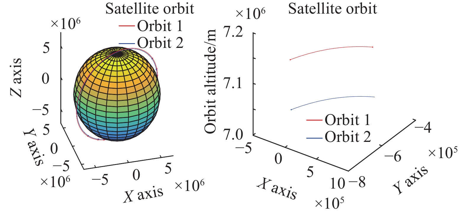
利用二体模型对高度为700 km和800 km的卫星轨道进行仿真,得到如图7所示的卫星轨道。

图 7 高度为700 km和800 km的卫星轨道及其局部放大图
Figure 7. Satellite orbits with heights of 700 km and 800 km and partial enlarged views
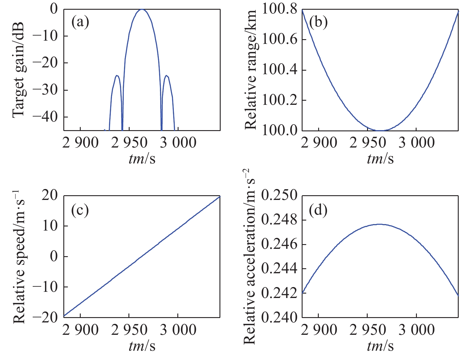
利用800 km轨道上的卫星1对700 km轨道上的卫星2进行SAL成像。当两低轨卫星运行方向相同时,卫星2的增益曲线如图8(a)所示,增益曲线的3 dB宽度为15个采样点,由于PRF的值不影响相干积累时间的计算,所以为节省程序运行时间,设置PRF为1 Hz,由图8(a)可知,卫星1对卫星2的最大相干积累时间为15 s。图8(b)、(c)和(d)分别为两卫星间的相对距离、相对速度和相对加速度变化曲线,由图可知,最大相干积累时间内两卫星间的相对距离最小为100 km、最大为100.01 km,相对速度变化较小,最大加速度不到0.25 m/s2,此时,可将两卫星间的相对运动看作做匀速直线运动。
图 8 两卫星运行方向相同时的成像参数(800 km/700 km)。(a)卫星2的增益曲线;(b)相对距离变化曲线;(c)相对速度变化曲线;(d)相对加速度变化曲线
Figure 8. Imaging parameters of two satellites in the same direction (800 km/700 km). (a) Gain curve of satellite 2; (b) Relative distance change curve; (c) Relative speed change curve; (d) Relative acceleration change curve
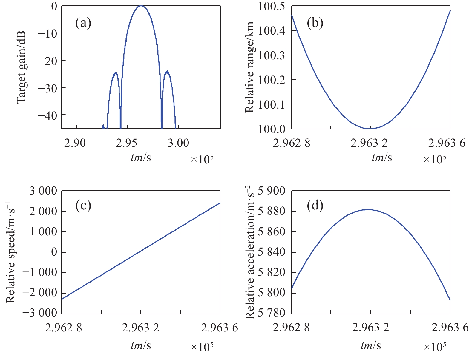
当两卫星运行方向相反时,卫星2的增益曲线如图9(a)所示,增益曲线的3 dB宽度为7个采样点,设置PRF为100 Hz,说明卫星1对卫星2的最大相干积累时间为0.07 s。图9(b)、(c)和(d)分别为两卫星间的相对距离、相对速度和相对加速度变化曲线,由图可知,最大相干积累时间内两卫星间的相对距离最小为100 km、最大为100.004 km,相对速度变化较大,最大加速度为5881 m/s2。
图 9 两卫星运行方向相反时的成像参数(800 km/700 km)。(a)卫星2的增益曲线;(b)相对距离变化曲线;(c)相对速度变化曲线;(d)相对加速度变化曲线
Figure 9. Imaging parameters of two satellites in the opposite direction (800 km/700 km). (a) Gain curve of satellite 2; (b) Relative distance change curve; (c) Relative speed change curve; (d) Relative acceleration change curve
-
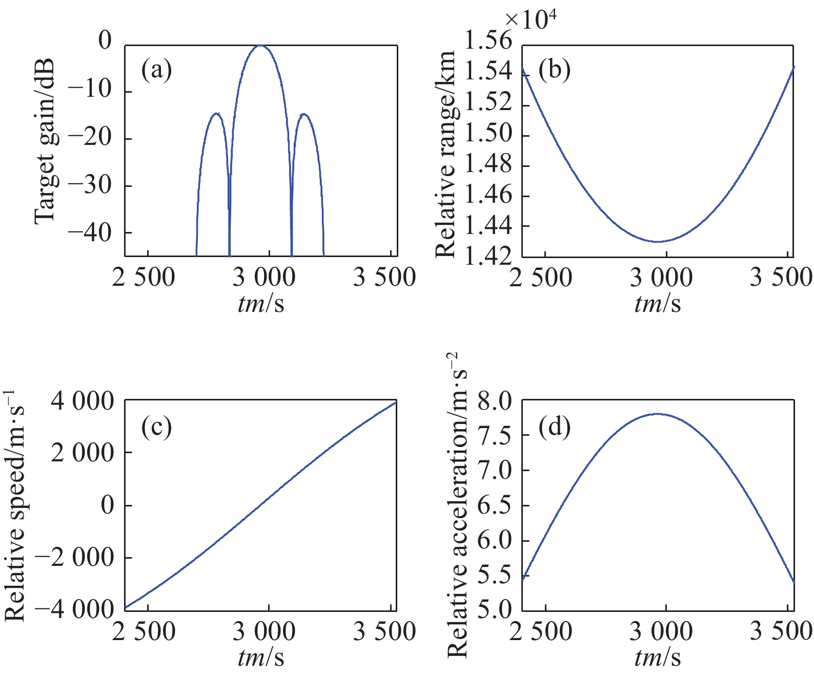
利用15 000 km轨道上的卫星1对700 km轨道上的卫星2进行SAL成像。当两卫星运行方向相同时,卫星2的增益曲线如图10(a)所示,增益曲线的3 dB宽度为111个采样点,设置PRF为1 Hz,说明卫星1对卫星2的最大相干积累时间为111 s。图10(b)、(c)和(d)分别为两卫星间的相对距离、相对速度和相对加速度变化曲线,由图可知,最大相干积累时间内两卫星间的相对距离最小为14 300 km、最大为14 312 km,最大加速度为7.79 m/s2。
图 10 两卫星运行方向相同时的成像参数(15000 km/700 km)。(a)卫星2的增益曲线;(b)相对距离变化曲线;(c)相对速度变化曲线;(d)相对加速度变化曲线
Figure 10. Imaging parameters of two satellites in the same direction (15000 km/700 km). (a) Gain curve of satellite 2; (b) Relative distance change curve; (c) Relative speed change curve; (d) Relative acceleration change curve
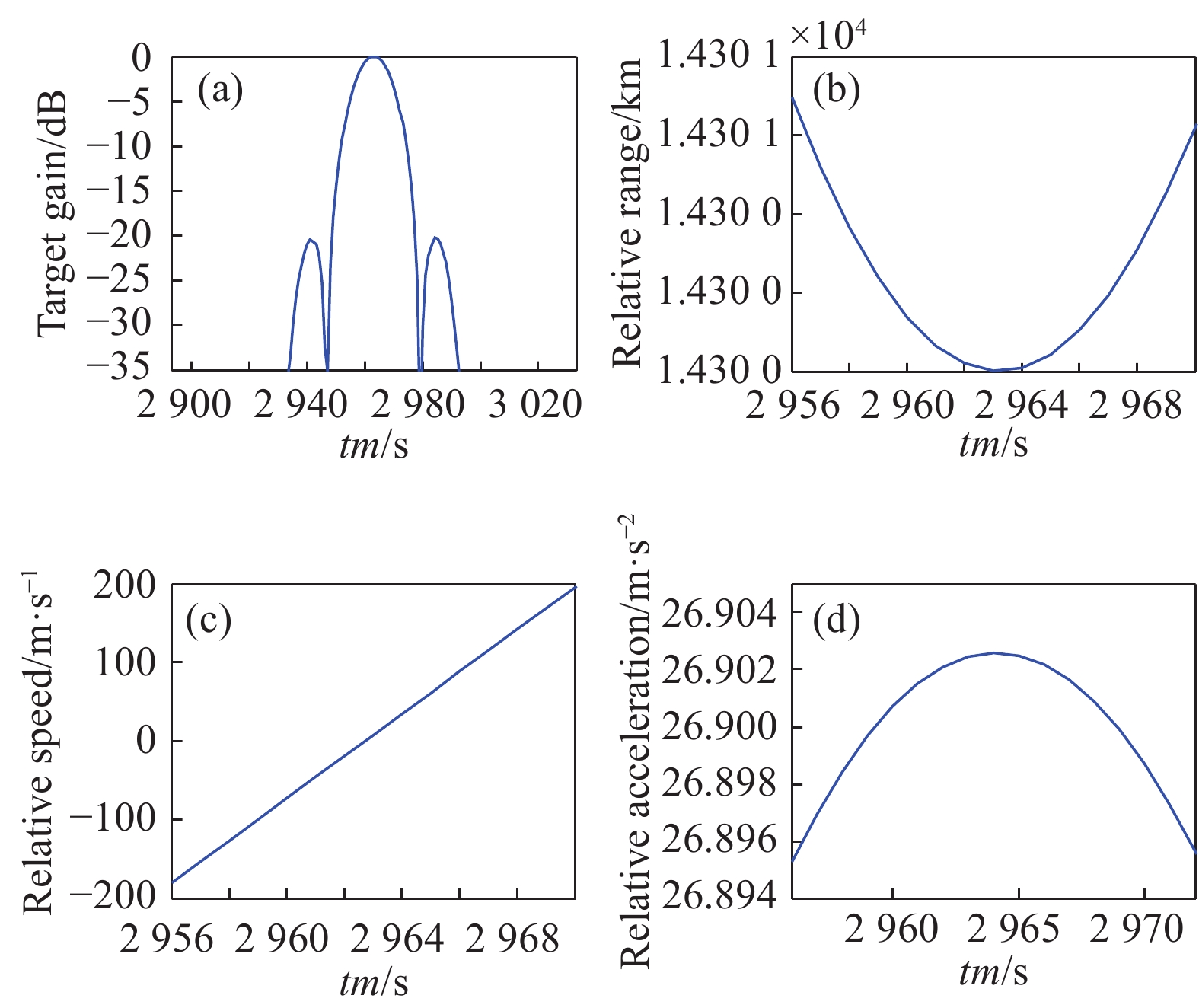
当两卫星运行方向相反时,卫星2的增益曲线如图11(a)所示,增益曲线的3 dB宽度为13个采样点,设置PRF为1 Hz,说明卫星1对卫星2的最大相干积累时间为13 s。图11(b)、(c)和(d)分别为两卫星间的相对距离、相对速度和相对加速度变化曲线,由图可知,最大相干积累时间内两卫星间的相对距离最小为14 300 km、最大为14 301 km,最大加速度为26.90 m/s2。
图 11 两卫星运行方向相反时的成像参数(15000 km/700 km)。(a)卫星2的增益曲线;(b)相对距离变化曲线;(c)相对速度变化曲线;(d)相对加速度变化曲线
Figure 11. Imaging parameters of two satellites in the opposite direction (15000 km/700 km). (a) Gain curve of satellite 2; (b) Relative distance change curve; (c) Relative speed change curve; (d) Relative acceleration change curve
-
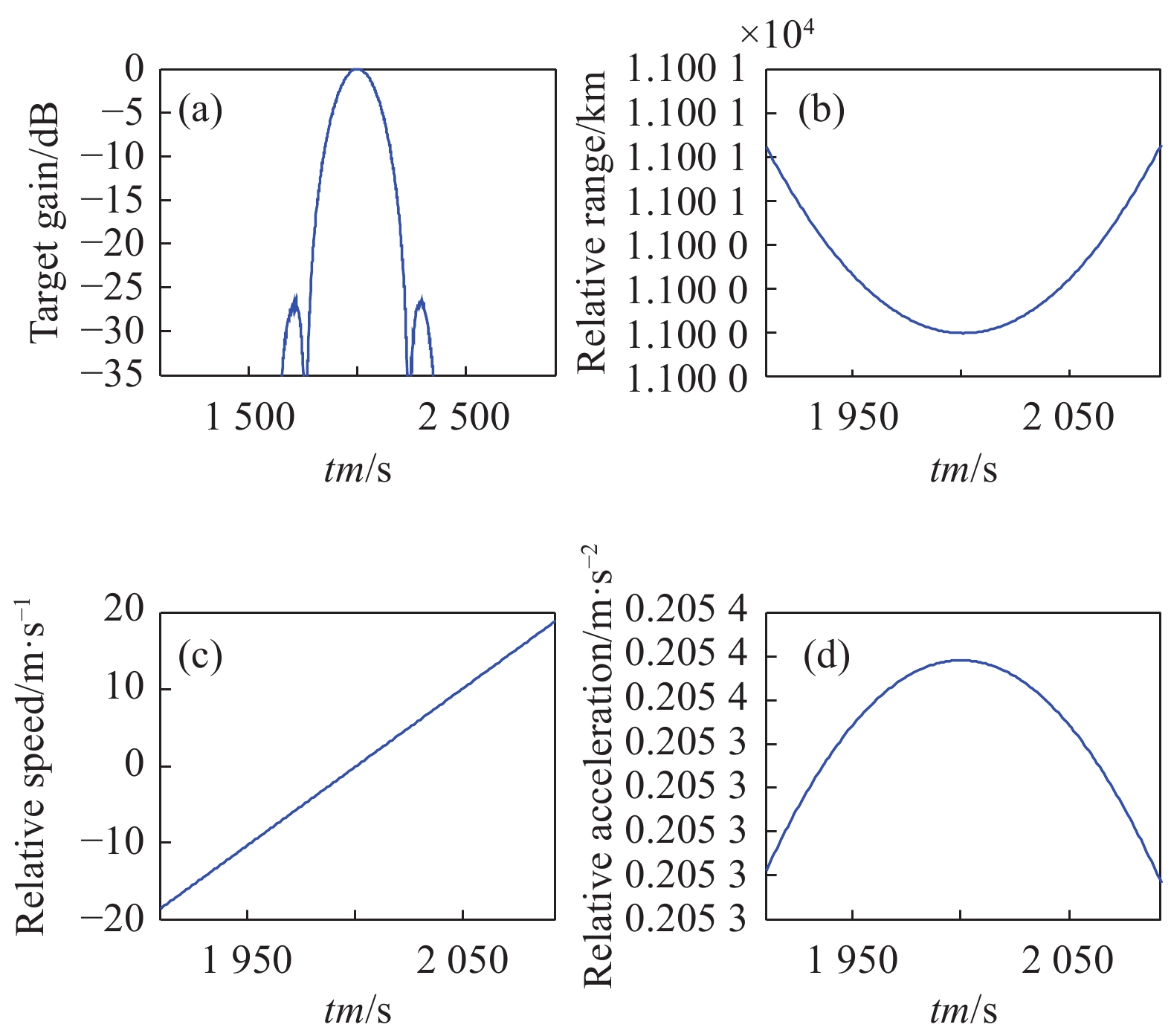
利用36000 km轨道上的卫星1对700 km轨道上的卫星2进行SAL成像。当两卫星运行方向相同时,卫星2的增益曲线如图12(a)所示,增益曲线的3 dB宽度为106个采样点,设置PRF为1 Hz,说明卫星1对卫星2的最大相干积累时间为106 s。图12(b)、(c)和(d)分别为两卫星间的相对距离、相对速度和相对加速度变化曲线,由图可知,最大相干积累时间内两卫星间的相对距离最小为35300 km、最大为35312 km,最大加速度为8.29 m/s2。
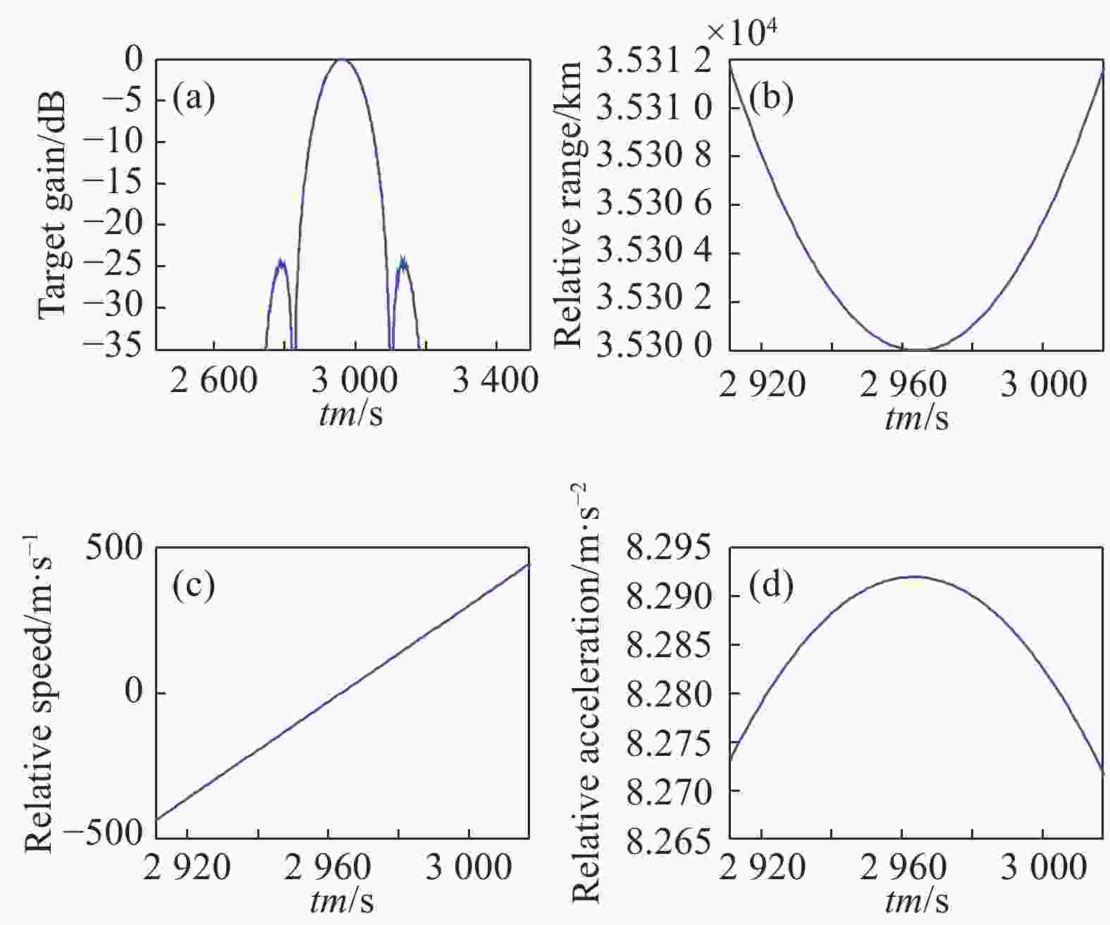
图 12 两卫星运行方向相同时的成像参数(36000 km/700 km)。(a)卫星2的增益曲线;(b)相对距离变化曲线;(c)相对速度变化曲线;(d)相对加速度变化曲线
Figure 12. Imaging parameters of two satellites in the same direction (36000 km/700 km). (a) Gain curve of satellite 2; (b) Relative distance change curve; (c) Relative speed change curve; (d) Relative acceleration change curve
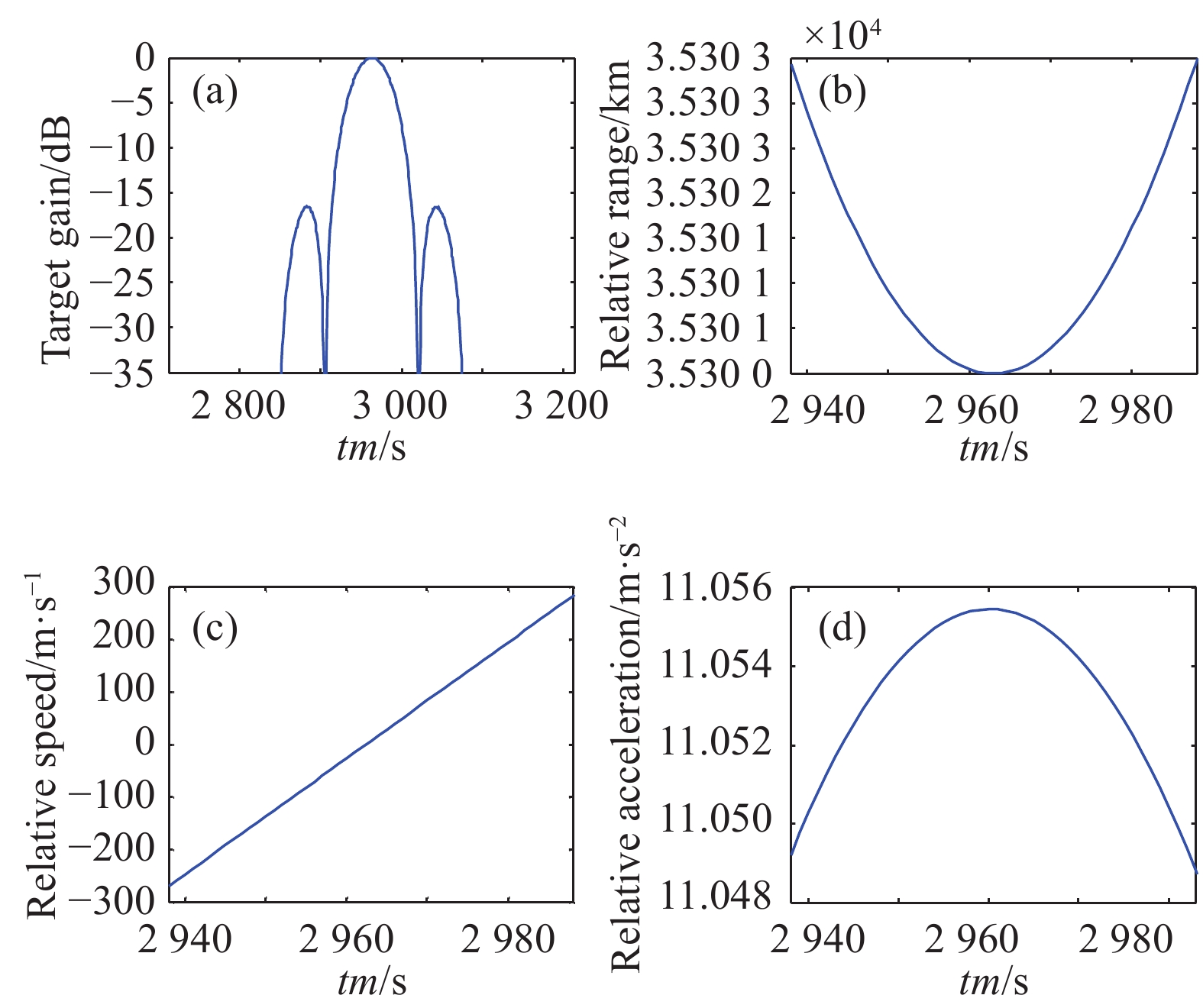
当两卫星运行方向相反时,卫星2的增益曲线如图13(a)所示,增益曲线的3 dB宽度为49个采样点,设置PRF为1 Hz,说明卫星1对卫星2的最大相干积累时间为49 s。图13(b)、(c)和(d)分别为两卫星间的相对距离、相对速度和相对加速度变化曲线,由图可知,最大相干积累时间内两卫星间的相对距离最小为35300 km、最大为35303 km,最大加速度为11.06 m/s2。

图 13 两卫星运行方向相反时的成像参数(36000 km/700 km)。(a)卫星2的增益曲线;(b)相对距离变化曲线;(c)相对速度变化曲线;(d)相对加速度变化曲线
Figure 13. Imaging parameters of two satellites in the opposite direction (36000 km/700 km). (a) Gain curve of satellite 2; (b) Relative distance change curve; (c) Relative speed change curve; (d) Relative acceleration change curve
-
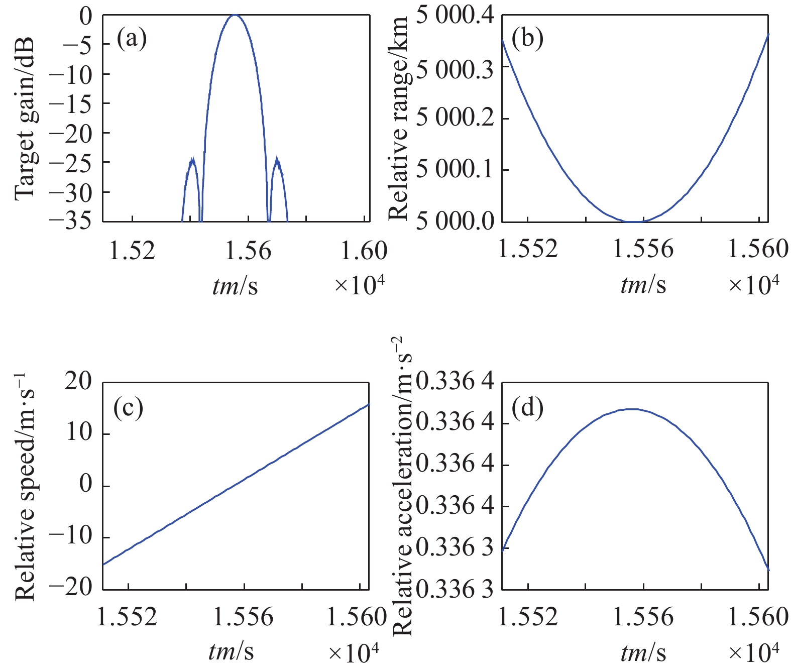
利用20000 km轨道上的卫星1对15000 km轨道上的卫星2进行SAL成像。当两卫星运行方向相同时,卫星2的增益曲线如图14(a)所示,增益曲线的3 dB宽度为91个采样点,设置PRF为1 Hz,说明卫星1对卫星2的最大相干积累时间为91 s。图14(b)、(c)和(d)分别为两卫星间的相对距离、相对速度和相对加速度变化曲线,由图可知,最大相干积累时间内两卫星间的相对距离最小5000 km、最大5000.4 km,相对速度变化较小,最大加速度为0.35 m/s2。
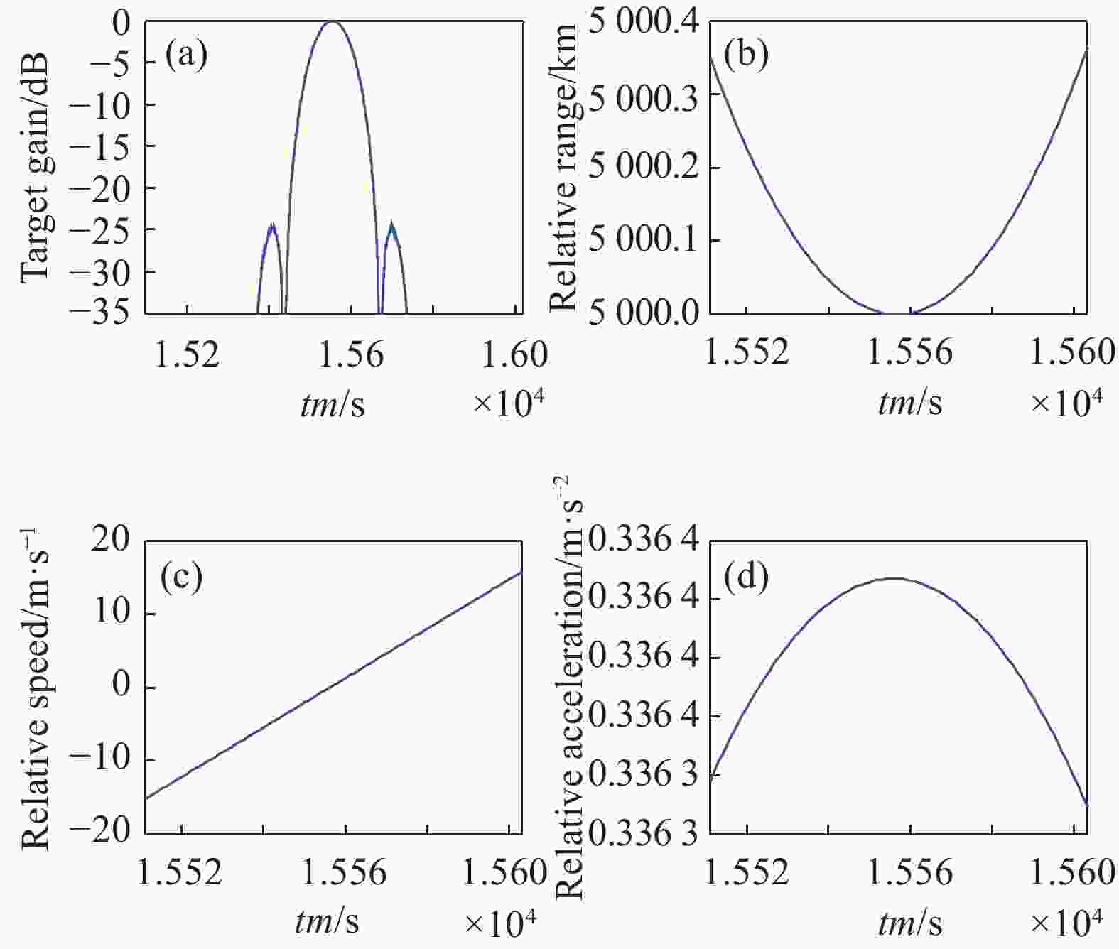
图 14 两卫星运行方向相同时的成像参数(20000 km/15000 km)。(a)卫星2的增益曲线;(b)相对距离变化曲线;(c)相对速度变化曲线;(d)相对加速度变化曲线
Figure 14. Imaging parameters of two satellites in the same direction (20000 km/15000 km). (a) Gain curve of satellite 2; (b) Relative distance change curve; (c) Relative speed change curve; (d) Relative acceleration change curve
当两卫星运行方向相反时,卫星2的增益曲线如图15(a)所示,增益曲线的3 dB宽度为7个采样点,设置PRF为1 Hz,说明卫星1对卫星2的最大相干积累时间为7 s。图15(b)、(c)和(d)分别为两卫星间的相对距离、相对速度和相对加速度变化曲线,由图可知,最大相干积累时间内两卫星间的相对距离最小为5000 km、最大为5000.2 km,最大加速度为23.31 m/s2。
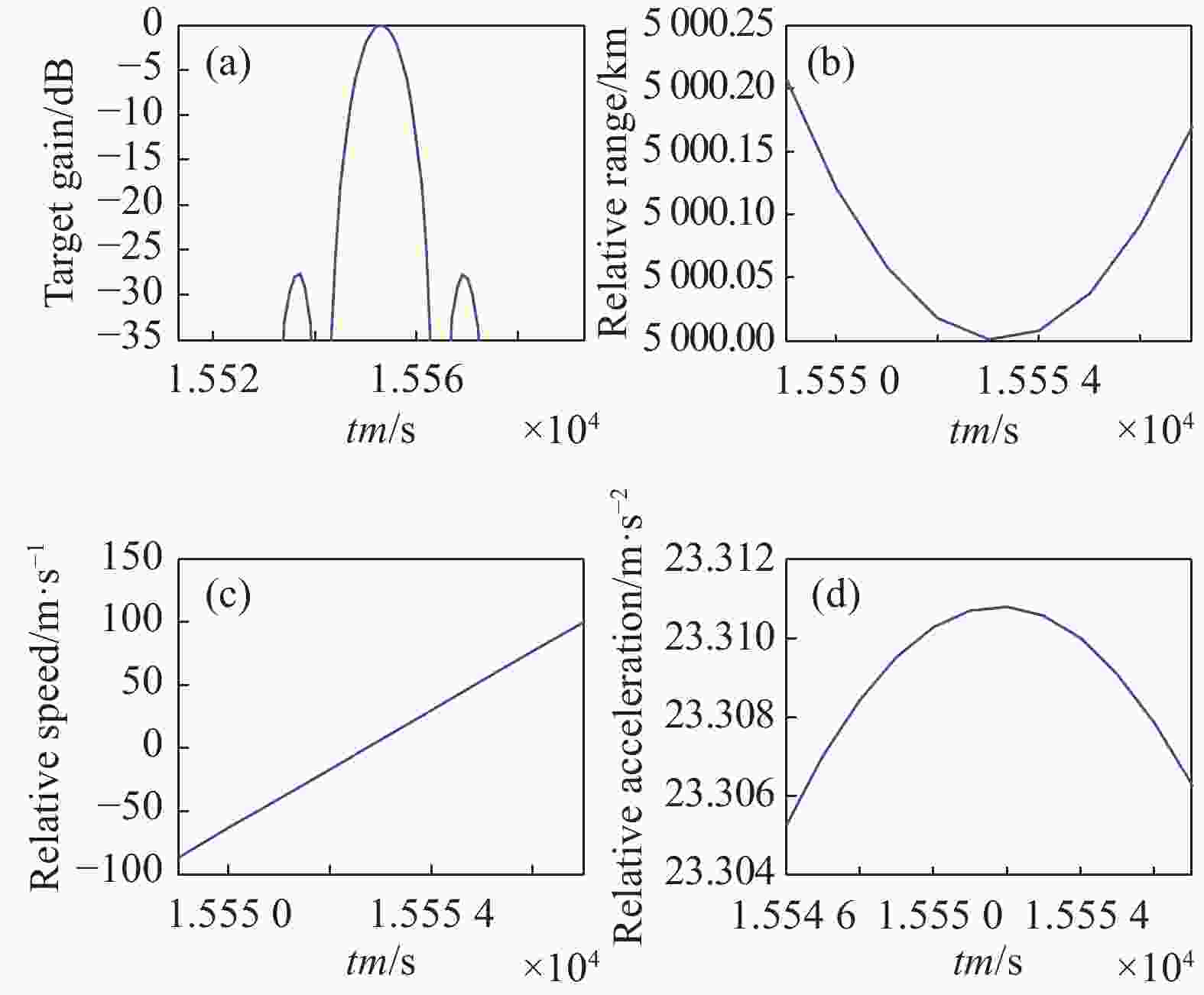
图 15 两卫星运行方向相反时的成像参数(20000 km/15000 km)。(a)卫星2的增益曲线;(b)相对距离变化曲线;(c)相对速度变化曲线;(d)相对加速度变化曲线
Figure 15. Imaging parameters of two satellites in the opposite direction (20000 km/15000 km). (a) Gain curve of satellite 2; (b) Relative distance change curve; (c) Relative speed change curve; (d) Relative acceleration change curve
-
利用36000 km轨道上的卫星1对15000 km轨道上的卫星2进行SAL成像。当两卫星运行方向相同时,卫星2的增益曲线如图16(a)所示,增益曲线的3 dB宽度为164个采样点,设置PRF为1 Hz,说明卫星1对卫星2的最大相干积累时间为164 s。图16(b)、(c)和(d)分别为两卫星间的相对距离、相对速度和相对加速度变化曲线,由图可知,最大相干积累时间内两卫星间的相对距离最小为2100 km、最大为2100.2 km,相对速度变化较小,最大加速度为0.72 m/s2。
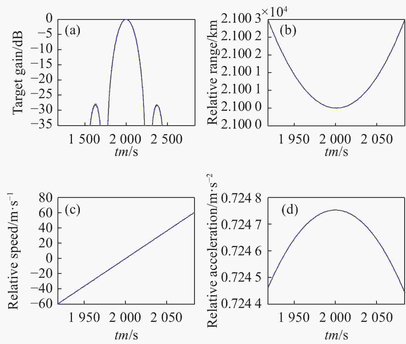
图 16 两卫星运行方向相同时的成像参数(36000 km/15000 km)。(a)卫星2的增益曲线;(b)相对距离变化曲线;(c)相对速度变化曲线;(d)相对加速度变化曲线
Figure 16. Imaging parameters of two satellites in the same direction (36000 km/15000 km). (a) Gain curve of satellite 2; (b) Relative distance change curve; (c) Relative speed change curve; (d) Relative acceleration change curve
当两卫星运行方向相反时,卫星2的增益曲线如图17(a)所示,增益曲线的3 dB宽度为38个采样点,设置PRF为1 Hz,说明卫星1对卫星2的最大相干积累时间为38 s。图17(b)、(c)和(d)分别为两卫星间的相对距离、相对速度和相对加速度变化曲线,由图可知,最大相干积累时间内两卫星间的相对距离最小为21000 km、最大为21001 km,最大加速度为4.12 m/s2。
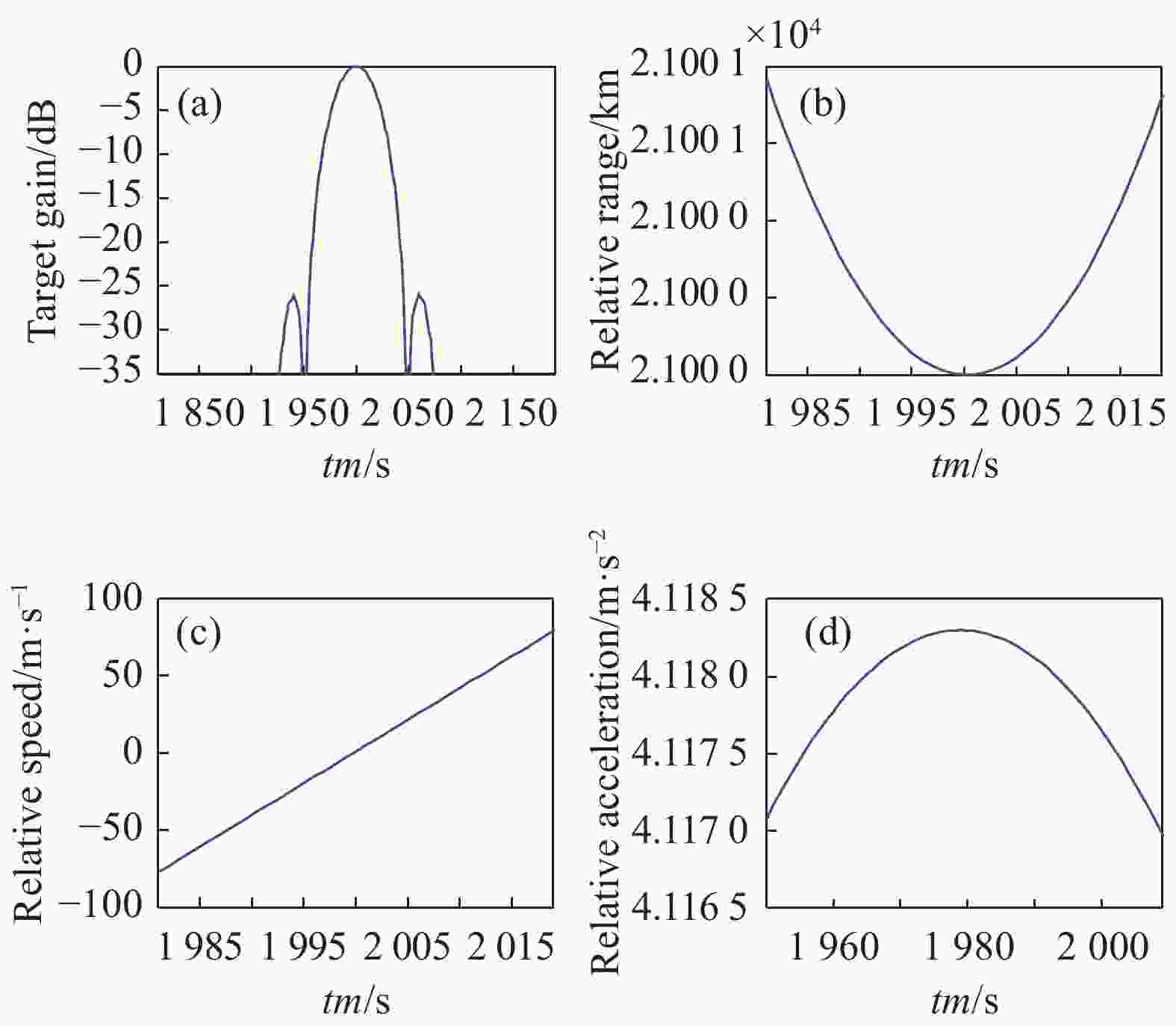
图 17 两卫星运行方向相反时的成像参数(36000 km/15000 km)。(a)卫星2的增益曲线;(b)相对距离变化曲线;(c)相对速度变化曲线;(d)相对加速度变化曲线
Figure 17. Imaging parameters of two satellites in the opposite direction (36000 km/15000 km). (a) Gain curve of satellite 2; (b) Relative distance change curve; (c) Relative speed change curve; (d) Relative acceleration change curve
-
利用36000 km轨道上的卫星1对25000 km轨道上的卫星2进行SAL成像。当两卫星运行方向相同时,卫星2的增益曲线如图18(a)所示,增益曲线的3 dB宽度为181个采样点,设置PRF为1 Hz,说明卫星1对卫星2的最大相干积累时间为181 s。图18(b)、(c)和(d)分别为两卫星间的相对距离、相对速度和相对加速度变化曲线,由图可知,最大相干积累时间内两卫星间的相对距离最小为11000 km、最大为11001 km,相对速度变化较小,最大加速度为0.21 m/s2。

图 18 两卫星运行方向相同时的成像参数(36000 km/25000 km)。(a)卫星2的增益曲线;(b)相对距离变化曲线;(c)相对速度变化曲线;(d)相对加速度变化曲线
Figure 18. Imaging parameters of two satellites in the same direction (36000 km/25000 km). (a) Gain curve of satellite 2; (b) Relative distance change curve; (c) Relative speed change curve; (d) Relative acceleration change curve
当两卫星运行方向相反时,卫星2的增益曲线如图19(a)所示,增益曲线的3 dB宽度为21个采样点,设置PRF为1 Hz,说明卫星1对卫星2的最大相干积累时间为21 s。图19(b)(c)和(d)分别为两卫星间的相对距离、相对速度和相对加速度变化曲线,由图可知,最大相干积累时间内两卫星间的相对距离变化较小为0.37 km,最大加速度为6.64 m/s2。
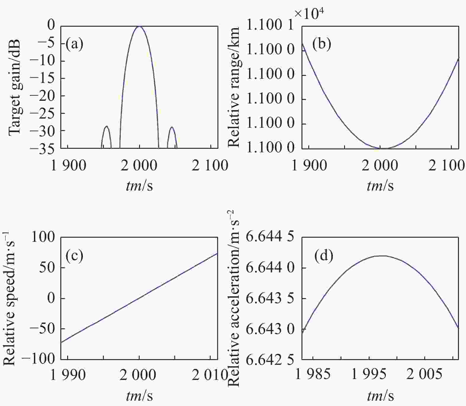
图 19 两卫星运行方向相反时的成像参数(36000 km/25000 km)。(a)卫星2的增益曲线;(b)相对距离变化曲线;(c)相对速度变化曲线;(d)相对加速度变化曲线
Figure 19. Imaging parameters of two satellites in the opposite direction (36000 km/25000 km). (a) Gain curve of satellite 2; (b) Relative distance change curve; (c) Relative speed change curve; (d) Relative acceleration change curve
为方便对比各模式下的成像参数,假设卫星天线长度为20 m,下面对各应用方式下的
$\Delta t$ (1064 nm波长、5 cm分辨率对应的相干积累时间)、最大相干积累时间、最大相干积累时间内两卫星间相对运动的最大加速度和多普勒带宽进行列表对比。对比下表可知,六种应用方式下的最大相干积累时间都是远大于
$\Delta t$ 的,说明天基SAL成像是可行的。从PRF选择的角度来说,PRF越小越好。为避免方位模糊,PRF的选择与
$\Delta {f_{\rm d}}$ 相关。根据公式(10)可知,两卫星轨道高度相差越小,$\Delta {f_{\rm d}}$ 的值越小,对PRF的要求也就越低。由表1可知,六种应用方式中,$\Delta {f_{\rm d}}$ 最小的是低轨对低轨且两卫星运行方向相同的成像方式,因为这种应用方式下的轨道高度差是所有应用方式中最小的。表 1 六种星对星SAL成像应用方式下的成像参数对比
Table 1. Comparison of imaging parameters in 6 SAL imaging applications
Imaging applications Orbit altitude /km Relative direction of
two satellites$\Delta t$/s Maximum
accumulation time/sMaximum relative
acceleration /m·s−2$\Delta {f_{\rm d}}$/kHz Low orbit satellite/
Low orbit satellite800/700 Same direction 0.007 15 0.25 0.830 Opposite direction 7.164e-5 0.07 5881 78.89 Medium orbit satellite/
Low orbit satellite15000/700 Same direction 0.025 111 7.79 32.27 Opposite direction 0.017 13 26.90 47.46 High orbit satellite/
Low orbit satellite36000/700 Same direction 0.054 106 8.29 37.14 Opposite direction 0.047 49 11.06 42.58 Medium orbit satellite/
Medium orbit satellite20000/15000 Same direction 0.046 91 0.35 2.06 Opposite direction 0.007 7 23.31 13.14 High orbit satellite/
Medium orbit satellite36000/15000 Same direction 0.081 164 0.72 4.88 Opposite direction 0.038 38 4.12 10.32 High orbit satellite/
High orbit satellite36000/25000 Same direction 0.091 181 0.21 1.55 Opposite direction 0.020 21 6.64 6.70 从合成孔径时间
$\Delta t$ 的角度来说,$\Delta t$ 越小越好,因为较长的$\Delta t$ 会带来较多不可预测的误差,比如卫星姿态误差等。由表1可知,六种应用方式中,$\Delta t$ 最小的是低轨对低轨且两卫星运行方向相反的成像方式,但是考虑到PRF的原因,认为最好的应用方式是低轨对低轨且两卫星运行方向相同的成像方式。根据表1可知,当两卫星的运行方向相同时,最大相干积累时间较两卫星运行方向相反时长,且此时两卫星间的加速度较小,因此,两卫星运行方向相同时,可等效为两卫星间做匀速直线运动,SAL成像时,对目标姿态估计可能比较复杂。当两卫星运行方向相反时,SAL成像所需的相干积累时间短,此时两卫星间的加速度较大,当由加速度引起的误差相位大于
$\pi /2$ 时,SAL成像的过程中,需要增加运动补偿部分。六种应用方式下方位向多普勒带宽
$\Delta {f_{\rm d}}$ 从几百Hz到几十kHz,相差较大。为了避免方位向模糊,PRF应大于$\Delta {f_{\rm d}}$ ,考虑到单通道模式下很难实现几十kHz的PRF,因此,对于大PRF的情况,可以采用单发多收或多发多收的方法实现。 -
本文对天基SAL成像进行了理论分析和仿真实验验证。利用天基SAL成像模型,推导出了天基SAL成像时相干积累时间与两卫星运行方向、两卫星轨道高度、图像分辨率和发射激光波长的关系。根据轨道六根数和二体运动轨道外推法,建立了卫星轨道模型,并利用该轨道模型,仿真了低轨对低轨、中轨对低轨、高轨对低轨、中轨对中轨、高轨对中轨和高轨对高轨的SAL应用方式。由于波束照射时间的影响,提出利用目标增益曲线的3 dB宽度,计算最大合成孔径时间的方法。最终,通过仿真分析不同应用方式下两卫星间的成像参数,验证了天基SAL成像的可行性,并为天基SAL成像算法的研究奠定了基础。
Parameters analysis of spaceborne synthetic aperture lidar imaging
-
摘要: 由于空间中没有大气,不存在大气湍流和大气衰减等问题,因此,相对于地基和机载合成孔径激光雷达(SAL),天基SAL有更好的应用前景。为验证中高低轨卫星间SAL成像的可行性,本文中建立了天基SAL成像模型,推导了星对星成像的相干积累时间和脉冲重复频率等参数。利用二体运动轨道外推法,建立了卫星轨道模型。并根据雷达天线波束宽度的限制,计算了激光雷达的收发天线方向图,提出利用目标增益曲线的3 dB波束宽度,获得最大合成孔径时间的方法。最后,通过仿真建立了六种天基SAL应用方式,并分析了不同应用方式下的成像参数,验证了天基SAL成像的可行性。本文的研究为天基SAL成像算法的研究奠定了基础。Abstract: Since there is no atmosphere in space, problems such as atmospheric turbulence and atmospheric attenuation do not exist. Therefore, spaceborne Synthetic Aperture Lidar (SAL) has a better application prospect than ground-based and airborne SAL. In order to verify the feasibility of airborne SAL imaging, a spaceborne SAL imaging model was established, and the coherent accumulation time and PRF were derived. Then, a satellite orbit model was established by using the extrapolation method of the two-body motion. Next, according to the limitation of the radar antenna beam width, the antenna pattern of the lidar was calculated, and a method to obtain the maximum synthetic aperture time was proposed by using the target gain curve's 3 dB beam width. Finally, six kinds of spaceborne SAL imaging modes were established through simulation, and the imaging parameters under different modes were analyzed, which verified the feasibility of spaceborne SAL imaging. The research of this paper lays a foundation for the research of spaceborne SAL imaging algorithm.
-
图 2 700 km高度轨道卫星的相干积累时间曲线。(a)两卫星运行方向相同;(b)两卫星运行方向相反
Figure 2. Coherent accumulation time curve of 700 km high orbit satellite. (a) Two satellites run in the same direction; (b) Two satellites run in opposite directions
图 3 15000 km高度轨道卫星的相干积累时间曲线。(a)两卫星运行方向相同;(b)两卫星运行方向相反
Figure 3. Coherent accumulation time curve of 15000 km high orbit satellite. (a) Two satellites run in the same direction; (b) Two satellites run in opposite directions
图 4 25000 km高度轨道卫星的相干积累时间曲线。(a)两卫星运行方向相同;(b)两卫星运行方向相反
Figure 4. Coherent accumulation time curve of 25000 km high orbit satellite. (a) Two satellites run in the same direction; (b) Two satellites run in opposite directions
图 6 天线方向图。(a)方位向一维天线方向图;(b)二维天线方向图
Figure 6. Antenna pattern. (a) Azimuth one-dimensional antenna pattern; (b) Two-dimensional antenna pattern
图 7 高度为700 km和800 km的卫星轨道及其局部放大图
Figure 7. Satellite orbits with heights of 700 km and 800 km and partial enlarged views
图 8 两卫星运行方向相同时的成像参数(800 km/700 km)。(a)卫星2的增益曲线;(b)相对距离变化曲线;(c)相对速度变化曲线;(d)相对加速度变化曲线
Figure 8. Imaging parameters of two satellites in the same direction (800 km/700 km). (a) Gain curve of satellite 2; (b) Relative distance change curve; (c) Relative speed change curve; (d) Relative acceleration change curve
图 9 两卫星运行方向相反时的成像参数(800 km/700 km)。(a)卫星2的增益曲线;(b)相对距离变化曲线;(c)相对速度变化曲线;(d)相对加速度变化曲线
Figure 9. Imaging parameters of two satellites in the opposite direction (800 km/700 km). (a) Gain curve of satellite 2; (b) Relative distance change curve; (c) Relative speed change curve; (d) Relative acceleration change curve
图 10 两卫星运行方向相同时的成像参数(15000 km/700 km)。(a)卫星2的增益曲线;(b)相对距离变化曲线;(c)相对速度变化曲线;(d)相对加速度变化曲线
Figure 10. Imaging parameters of two satellites in the same direction (15000 km/700 km). (a) Gain curve of satellite 2; (b) Relative distance change curve; (c) Relative speed change curve; (d) Relative acceleration change curve
图 11 两卫星运行方向相反时的成像参数(15000 km/700 km)。(a)卫星2的增益曲线;(b)相对距离变化曲线;(c)相对速度变化曲线;(d)相对加速度变化曲线
Figure 11. Imaging parameters of two satellites in the opposite direction (15000 km/700 km). (a) Gain curve of satellite 2; (b) Relative distance change curve; (c) Relative speed change curve; (d) Relative acceleration change curve
图 12 两卫星运行方向相同时的成像参数(36000 km/700 km)。(a)卫星2的增益曲线;(b)相对距离变化曲线;(c)相对速度变化曲线;(d)相对加速度变化曲线
Figure 12. Imaging parameters of two satellites in the same direction (36000 km/700 km). (a) Gain curve of satellite 2; (b) Relative distance change curve; (c) Relative speed change curve; (d) Relative acceleration change curve
图 13 两卫星运行方向相反时的成像参数(36000 km/700 km)。(a)卫星2的增益曲线;(b)相对距离变化曲线;(c)相对速度变化曲线;(d)相对加速度变化曲线
Figure 13. Imaging parameters of two satellites in the opposite direction (36000 km/700 km). (a) Gain curve of satellite 2; (b) Relative distance change curve; (c) Relative speed change curve; (d) Relative acceleration change curve
图 14 两卫星运行方向相同时的成像参数(20000 km/15000 km)。(a)卫星2的增益曲线;(b)相对距离变化曲线;(c)相对速度变化曲线;(d)相对加速度变化曲线
Figure 14. Imaging parameters of two satellites in the same direction (20000 km/15000 km). (a) Gain curve of satellite 2; (b) Relative distance change curve; (c) Relative speed change curve; (d) Relative acceleration change curve
图 15 两卫星运行方向相反时的成像参数(20000 km/15000 km)。(a)卫星2的增益曲线;(b)相对距离变化曲线;(c)相对速度变化曲线;(d)相对加速度变化曲线
Figure 15. Imaging parameters of two satellites in the opposite direction (20000 km/15000 km). (a) Gain curve of satellite 2; (b) Relative distance change curve; (c) Relative speed change curve; (d) Relative acceleration change curve
图 16 两卫星运行方向相同时的成像参数(36000 km/15000 km)。(a)卫星2的增益曲线;(b)相对距离变化曲线;(c)相对速度变化曲线;(d)相对加速度变化曲线
Figure 16. Imaging parameters of two satellites in the same direction (36000 km/15000 km). (a) Gain curve of satellite 2; (b) Relative distance change curve; (c) Relative speed change curve; (d) Relative acceleration change curve
图 17 两卫星运行方向相反时的成像参数(36000 km/15000 km)。(a)卫星2的增益曲线;(b)相对距离变化曲线;(c)相对速度变化曲线;(d)相对加速度变化曲线
Figure 17. Imaging parameters of two satellites in the opposite direction (36000 km/15000 km). (a) Gain curve of satellite 2; (b) Relative distance change curve; (c) Relative speed change curve; (d) Relative acceleration change curve
图 18 两卫星运行方向相同时的成像参数(36000 km/25000 km)。(a)卫星2的增益曲线;(b)相对距离变化曲线;(c)相对速度变化曲线;(d)相对加速度变化曲线
Figure 18. Imaging parameters of two satellites in the same direction (36000 km/25000 km). (a) Gain curve of satellite 2; (b) Relative distance change curve; (c) Relative speed change curve; (d) Relative acceleration change curve
图 19 两卫星运行方向相反时的成像参数(36000 km/25000 km)。(a)卫星2的增益曲线;(b)相对距离变化曲线;(c)相对速度变化曲线;(d)相对加速度变化曲线
Figure 19. Imaging parameters of two satellites in the opposite direction (36000 km/25000 km). (a) Gain curve of satellite 2; (b) Relative distance change curve; (c) Relative speed change curve; (d) Relative acceleration change curve
表 1 六种星对星SAL成像应用方式下的成像参数对比
Table 1. Comparison of imaging parameters in 6 SAL imaging applications
Imaging applications Orbit altitude /km Relative direction of
two satellites$\Delta t$ /sMaximum
accumulation time/sMaximum relative
acceleration /m·s−2$\Delta {f_{\rm d}}$ /kHzLow orbit satellite/
Low orbit satellite800/700 Same direction 0.007 15 0.25 0.830 Opposite direction 7.164e-5 0.07 5881 78.89 Medium orbit satellite/
Low orbit satellite15000/700 Same direction 0.025 111 7.79 32.27 Opposite direction 0.017 13 26.90 47.46 High orbit satellite/
Low orbit satellite36000/700 Same direction 0.054 106 8.29 37.14 Opposite direction 0.047 49 11.06 42.58 Medium orbit satellite/
Medium orbit satellite20000/15000 Same direction 0.046 91 0.35 2.06 Opposite direction 0.007 7 23.31 13.14 High orbit satellite/
Medium orbit satellite36000/15000 Same direction 0.081 164 0.72 4.88 Opposite direction 0.038 38 4.12 10.32 High orbit satellite/
High orbit satellite36000/25000 Same direction 0.091 181 0.21 1.55 Opposite direction 0.020 21 6.64 6.70  下载: 导出CSV
-
[1] Funk E, Reintjes J, Rickard L J, et al. Two -dimensional synthetic aperture imaging in the optical domain [J]. Optics Letters, 2002, 27(22): 1983-1985. doi: 10.1364/OL.27.001983 [2] Ricklin J, Schumm B, Dierking M, et al. Synthetic aperture ladar for tactical imaging[R]. US: DARPA Strategic Technology Office, 2007. [3] 邢孟道, 郭亮, 唐禹, 等. 室内实测数据的逆合成孔径激光雷达成像[J]. 红外与激光工程, 2009, 38(2): 290-294. doi: 10.3969/j.issn.1007-2276.2009.02.022 Xing Mengdao, Guo Liang, Tang Yu, et al. Design on the experiment optical system of synthetic aperture imaging lidar [J]. Infrared and Laser Engineering, 2009, 38(2): 290-294. (in Chinese) doi: 10.3969/j.issn.1007-2276.2009.02.022 [4] 周煜, 许楠, 栾竹, 等. 尺度缩小合成孔径激光雷达的二维成像实验[J]. 光学学报, 2009, 29(7): 2030-2032. doi: 10.3788/AOS20092907.2030 Zhou Yu, Xu Nan, Luan Zhu, et al. 2D imaging experiment of a 2D target in a laboratory-scale synthetic aperture imaging ladar [J]. Acta Optica Sinica, 2009, 29(7): 2030-2032. (in Chinese) doi: 10.3788/AOS20092907.2030 [5] Croch S, Barber Z W. Laboratory demonstration of interferometric and spotlight synthetic aperture ladar techniques [J]. Optics Express, 2012, 20(22): 24237-24246. doi: 10.1364/OE.20.024237 [6] Turbide S, Marchese L, Bergeron A, et al. Synthetic aperture ladar based on a MOPAW laser[C]. Remote Sensing, 2016. [7] Krause B W, Buck J, Ryan C, et al. Synthetic aperture ladar flight demonstration[C]//Quantum Electronics and Laser Science Conference, 2011: PDPB7. [8] Li G Z, Wang N, Wang R, et a;. Imaging method for airborne SAL data [J]. Electronics Letters, 2017, 53(5): 351-353. doi: 10.1049/el.2016.4205 [9] 卢智勇, 周煜, 孙建锋, 等. 机载直视合成孔径激光成像雷达外场及飞行试验[J]. 中国激光, 2017, 44(1): 0110001. doi: 10.3788/CJL201744.0110001 Lu Zhiyong, Zhou Yu, Sun Jianfeng, et al. Airborne down-looking synthetic aperture imaging ladar field experiment and flight testing [J]. Chinese Journal of Laser, 2017, 44(1): 0110001. (in Chinese) doi: 10.3788/CJL201744.0110001 [10] 李道京, 杜剑波, 马萌, 等. 天基合成孔径激光雷达系统分析[J]. 红外与激光工程, 2016, 45(11): 113002. Li Daojing, Du Jianbo, Ma Meng, et al. Synthetic analysis of spaceborn synthetic aperture ladar [J]. Infrared and Laser Engineering, 2016, 45(11): 113002. (in Chinese) [11] 阮航, 吴彦鸿, 张书仙, 等. 基于天基逆合成孔径激光雷达的静止轨道目标成像[J]. 红外与激光工程, 2013, 42(6): 1611-1616. doi: 10.3969/j.issn.1007-2276.2013.06.041 Ruan Hang, Wu Yanhong, Zhang Shuxian. Geostationary orbital object imaging based on spaceborne inverse synthetic aperture ladar [J]. Infrared and Laser Engineering, 2013, 42(6): 1611-1616. (in Chinese) doi: 10.3969/j.issn.1007-2276.2013.06.041 [12] 李道京, 朱宇, 胡烜, 等. 衍射光学系统的激光应用和稀疏成像分析[J]. 雷达学报, 2020, 9(1): 195-230. doi: 10.12000/JR19081 Li Daojing, Zhu Yu, Hu Xuan, et al. Lasar application and sparse imaging analysis of diffractive optical system [J]. Journal of Radars, 2020, 9(1): 195-230. (in Chinese) doi: 10.12000/JR19081 [13] Li Jinming, Hu Yihua, Li Jinshan, et al. Orbit of spaceborne SAL for geostationary satellites imaging [J]. Infrared and Laser Engineering, 2012, 41(3): 684-689. (in Chinese) [14] 李丹阳, 吴谨, 万磊, 等. 天基合成孔径激光雷达成像理论初步[J]. 光学学报, 2019, 39(7): 0728002. Li Danyang, Wu Jin, Wang Lei, et al. Elementary imaging theory in space_borne synethetic aperture ladar [J]. Acta Optica Sinica, 2019, 39(7): 0728002. (in Chinese) [15] 李飞, 张鸿翼, 徐卫明, 等. 天基合成孔径激光雷达非合作目标成像系统设计与实验[J]. 红外与激光工程, 2016, 45(10): 1030001. doi: 10.3788/IRLA201645.1030001 Li Fei, Zhang Hongyi, Xu Weiming, et al. Design and experiment of space borne synthetic aperture ladar for non-cooperative targets imaging system [J]. Infrared and Laser Engineering, 2016, 45(10): 1030001. (in Chinese) doi: 10.3788/IRLA201645.1030001 [16] 丁鹭飞, 耿富录. 雷达原理[M]. 西安: 西安电子科技大学出版社, 1995. Ding Lufei, Geng Fulu. Radar Principle[M]. Xi'an: Xidian University Press, 1995. [17] 魏钟铨, 吴一戎, 王长耀, 等. 合成孔径雷达卫星[M]. 北京: 科学出版社, 2001. Wei Zhongquan, Wu Yirong, Wang Changyao, et al. SAR Satellite[M]. Beijing: Science Press, 2001. (in Chinese) [18] Zhang Guangyi, Zhao Yujie, Wang Xiaomo, et al. Phase Array Radar Technology[M]. Beijing: Electronic Industry Press, 2006. (in Chinese) -

 点击查看大图
计量
- 文章访问数: 766
- HTML全文浏览量: 215
- PDF下载量: 82
- 被引次数: 0


