


-
随着超精密加工技术、极紫外光刻技术(EUV)、纳机电系统(NEMS)为代表的加工技术和工艺的快速发展,半导体产业中的纳米器件和结构尺寸越做越小、薄膜厚度变得越来越薄,对薄膜厚度等参数的精确测量要求越来越高[1-3]。目前,半导体产业中用作栅极氧化层的超薄薄膜厚度的偏差要求为5%~10%左右,对各种薄膜厚度参数的精确测量与溯源性分析是保证器件质量、提高生产效率的重要手段[4]。原子力显微镜(AFM)和扫描电子显微镜(SEM)是可以将纳米结构可视化的传统仪器,但是却不适合实时在线监测制造的过程[5],椭圆偏振法是一种可以对纳米样板实现高效率的测量和信息传输的测量方法。与自然光相比,偏振光可以具有包括偏振态在内的更多信息,测量时可以通过被测物体反射光偏振态的变化来获得薄膜和纳米图案的光学和几何特性。与传统的纳米测量方法相比,椭偏法不仅具有操作简单、测量精度高等优点,同时可以实现非接触无损测量。随着纳米技术的不断发展,特别是在薄膜厚度小于光波长的情况下,椭偏法更体现出其重要性[6]。
虽然椭偏法相较于其他测量法已经是高精度的测量方法,但在操作中难免会产生的系统和随机误差[3]。所以为了保证测量精度,需要对测量系统中的元件参数进行定标。作为纳米级高精度的测量仪器,椭偏仪的定标具有一定难度,近年来逐渐成为量子光学领域的研究热点。传统的定标方法主要有E-P定标法和四点定标法[7-8],然而这两种方法都没有考虑光源自身的偏振效应和偏振器件产生误差,影响定标精度。椭偏系统中各个元器件都是独立的,在考虑偏振器件方位角误差和延迟误差的基础上,用列文伯格-马夸尔特(LM)算法求解偏振光传输系统的非线性多元拟合方程中的基本元件参数,从而实现表征测量系统[9-11]。
基于以上分析,文中将通过对测量系统中元件参数的建模和求解实现标定,通过对穆勒椭偏测量系统进行实验,验证方法的可行性。并通过对标准样品膜厚的测量验证光学元件参数值的有效性,实现椭偏系统快速、高精度的定标。
-
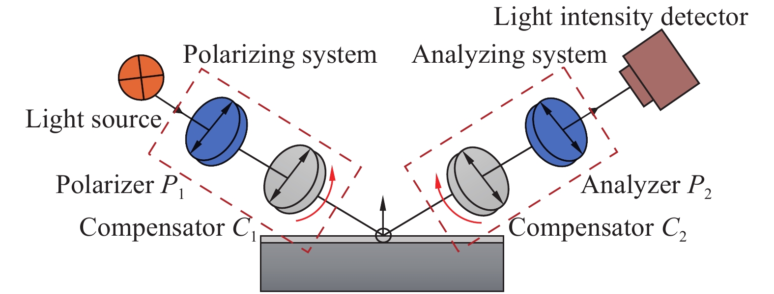
椭偏仪是凭借测量经过样品散射后光束偏振态的变化,通过建模和计算,反演出被测样品的膜厚和光学特性[12]。测量过程主要有两步:一是通过正向光学建模,构建样品膜层、膜厚等几何参数以及光源入射角、偏振器方位角之间的理论光强矩阵;二是通过搭建的穆勒椭偏系统测量样品的实际光强矩阵,并与模型计算的理论光矩阵匹配,满足精度的情况下提取参数。光束在椭偏仪中的光路如图1所示[1]。
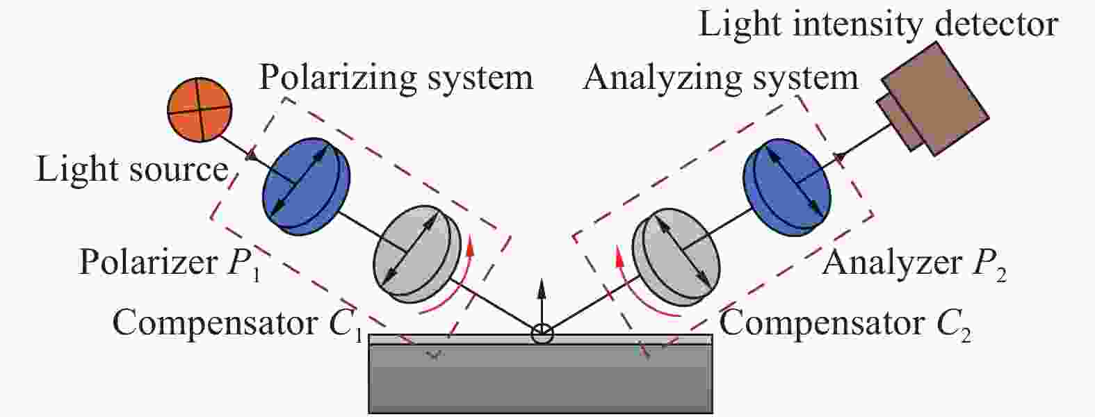
图 1 光束在椭偏系统中的光路图
Figure 1. Light path diagram of light beam in ellipsoidal system
整个测量系统由光源、起偏器系统、样品、检偏系统和光强探测器组成。从光源出射的平行光束经过起偏器P1变成偏振光,进入补偿器C1进行相位调制,然后以入射角θ入射到样品表面,经样品反射后进入C2进行相位解调,然后经过检偏器P2,由光强探测器D进行数据的采集。为了得到不同状态的入射光,电机带动起偏系统的补偿器C1和检偏系统的补偿器C2各自以一定步长n1和n2独立旋转,系统中补偿器C1和补偿器C2以1:5的转速比同步旋转。光束在系统中的变化过程可以用元件的传输矩阵表示[13]:
$$ {S_{out}} = E{M_P}{M_{{C_2}}}{M_{{\text{样品}}}}{M_{{C_1}}}{M_A}{S_{in}} $$ (1) 式中:Sin为入射光的斯托克斯矢量;Sout为入射光和出射光的斯托克斯矢量,均为无量纲的。Mueller矩阵中的16个元素都有具体的物理意义,其中m00只包含光强信息,通常为了直观的表示光束的偏振态,对光束的斯托克斯矢量进行归一化处理[14-15]。其中MP、MA、MC1
、MC2分别为起偏器、旋转波片、检偏器的Mueller矩阵。 理想条件下,椭偏系统中起偏器、检偏器和两个旋转相位补偿器的Mueller矩阵如下[16]:
$$ {M_P}{\rm{ = }}R\left( { - P} \right){M_P} = \dfrac{1}{2}\left( {\begin{array}{*{20}{c}} 1&{\cos 2P}&{\sin 2P}&0\\ {\cos 2P}&{{{\cos }^2}2P}&{\sin 2P\cos 2P}&0\\ {\sin 2P}&{\sin 2P\cos 2P}&{{{\sin }^2}2P}&0\\ 0&0&0&0 \end{array}} \right) $$ (2) $$ {M_A} = {M_A}R\left( A \right){\rm{ = }}\dfrac{1}{2}\left( {\begin{array}{*{20}{c}} 1&{\cos 2A}&{\sin 2A}&0\\ {\cos 2A}&{{{\cos }^2}2A}&{\sin 2A\cos 2A}&0\\ {\sin 2A}&{\sin 2A\cos 2A}&{{{\sin }^2}2A}&0\\ 0&0&0&0 \end{array}} \right) $$ (3) $$ \begin{array}{l} {M_{{C_1}}} = R\left( { - {C_1}} \right){M_{{c_1}}}\left( {{\Delta _1}} \right)R\left( {{C_1}} \right) = \\ \left( {\begin{array}{*{20}{c}} 1&0&0&0\\ 0&{1 - \left( {1 - \cos {\Delta _1}} \right){{\sin }^2}2{C_1}}&{\left( {1 - \cos {\Delta _1}} \right)\sin 2{C_1}\cos 2{C_1}}&{ - \sin {\Delta _1}\sin 2{C_1}}\\ 0&{\left( {1 - \cos {\Delta _1}} \right)\sin 2{C_1}\cos 2{C_1}}&{1 - \left( {1 - \cos {\Delta _1}} \right){{\cos }^2}2{C_1}}&{\cos {\Delta _1}\cos 2{C_1}}\\ 0&{\sin {\Delta _1}\sin 2{C_1}}&{ - \sin {\Delta _1}\cos 2{C_1}}&{\cos {\Delta _1}} \end{array}} \right) \end{array} $$ (4) $$ \begin{array}{l} {M_{{C_2}}} = R\left( { - {C_2}} \right){M_{{c_1}}}\left( {{\Delta _2}} \right)R\left( {{C_2}} \right) = \\ \left( {\begin{array}{*{20}{c}} 1&0&0&0\\ 0&{1 - \left( {1 - \cos {\Delta _2}} \right){{\sin }^2}2{C_2}}&{\left( {1 - \cos {\Delta _2}} \right)\sin 2{C_2}\cos 2{C_2}}&{ - \sin {\Delta _2}\sin 2{C_2}}\\ 0&{\left( {1 - \cos {\Delta _2}} \right)\sin 2{C_2}\cos 2{C_2}}&{1 - \left( {1 - \cos {\Delta _2}} \right){{\cos }^2}2{C_2}}&{\cos {\Delta _2}\cos 2{C_2}}\\ 0&{\sin {\Delta _2}\sin 2{C_2}}&{ - \sin {\Delta _2}\cos 2{C_2}}&{\cos {\Delta _2}} \end{array}} \right) \end{array} $$ (5) 式中:A和P为起偏器和检偏器的方位角;Δ1和Δ2为1/4旋转波片C1和C2的相位延迟,假设波片C1和C2的初始方位角为c1
和c2 ;t为采样时刻。则两片波片旋转时相位: $${C_1} = \omega t - {c_1};\;{C_2} = 5(\omega t - {c_2})$$ (6) 在一个旋转周期(π)内,在相同的时间间隔内采集I,共可以采集到(360º/n1)*(360º/n2)组光强。将公式(2)~(6)代入公式(1)中。在红外椭偏测量系统中,出射光斯托克斯矢量的第一个元素Sout(1,1)为光强探测器测量的光强值。所以出射光强只与中间据矩阵MP、
MC2、MS、 MC1 、MA乘积矩阵的第一行元素有关,可以建立出射光与椭偏系统中所有未知参量的非线性方程: $$ \begin{split} {I_{out}} =& E{M_P}{M_{{C_2}}}{M_S}{M_{{C_1}}}{M_A}{S_{in}}=\\ & {{ F}}\left( {\left( {{s_0},{s_1},{s_2},{s_3},A,P,{c_1},{c_2},{\Delta _1},{\Delta _2}} \right),{M_{{\text{样品}}}}} \right) \end{split} $$ (7) 公式(7)是一个非线性参数,且含有较多的未知参数,是一个典型的回归问题,可以通过拟合法求参数。
-
模型求出的光强与实际测量的光强会存在一定的残差,要使模型的总残差最小,本质上是一个全局最优化问题。非线性最小二乘是解决非线性、多参数的复杂函数最优解的算法,可以用来拟合参数。
-
在放置已知Mueller矩阵的标准样片时,系统中的未知参数只有元器件参数。待拟合参数为起偏器的方位角A和检偏器的方位角P,旋转波片C1
、C2 的初始方位角c1 和c2 ,波片的相位延迟Δ1 和Δ2 。自变量为入射光的斯托克斯矢量Sin,应变量为出射光测量值和模拟值的残差y。 将非线性参数集{A, P, c1
, c2, Δ1, Δ2}内的参数进行标号,记为非线性参数集X:{u1 , u2, u3, u4, u5, u6},自变量入射光集Sini标为{x1, x2, x3,….},应变量出射光集Souti标为{y1, y2, y3,….}。 $$ \begin{split} {\chi ^2} = \phi \left( {{u_j}} \right) =& \min \left[ {\sum\limits_{i = 1}^{{{360}^ \circ }/n} {{{\left( {{I_t}_i - {I_{outi}}} \right)}^2}} } \right] =\\ & \min \left[ {\sum\limits_{i = 1}^{{{360}^ \circ }/n} {{y_i}^2} } \right] =\\ & \min f \end{split} $$ (8) 式中:i=1,2,…, m为样本点数量;j为待优化参数的维度。根据最小二乘法的原则
$\partial {\phi _i}/\partial {u_j} = 0$ ,通过迭代求得具有最小残差平方和的参数值。假设系统出射光的实际测量值为S,与模型的估计值Sout残差为y。假设残差的平方和为χ2,根据最大似然估计和高斯分布的特点,最小化残差和等价于最小化残差的平方和:
$$\phi \left( {x;{u_j}} \right) = \dfrac{{{\chi ^2}}}{2}{\rm{ = }}\dfrac{{\displaystyle \sum\limits_{i = 1}^{{{360}^ \circ }/n} {{y_i}^2} }}{2}$$ (9) 公式(9)为优化目标函数,函数关于参数ui的一阶导数:
$$\dfrac{{\partial \phi }}{{\partial {u_j}}}{\rm{ = }}\dfrac{\partial }{{\partial {u_j}}}\dfrac{1}{2}\sum\limits_{i = 1}^m {y_i^2} = \sum\limits_{i = 1}^m {{y_i}\dfrac{{\partial {y_i}}}{{\partial {u_j}}}} $$ (10) $\phi $ 的一阶导数用Hamiltonian算子表示:$$\nabla \phi {\rm{ = }}{J_y}{\left( u \right){\rm{^T}}}y\left( u \right)$$ (10) 其中,yi对参数的雅克比矩阵(Jacobian) Jy(u):
$${J_y}\left( u \right) = \dfrac{{\partial {y_i}}}{{\partial {u_j}}}\left[ {\begin{array}{*{20}{c}} {\dfrac{{\partial {y_1}}}{{\partial {u_1}}}}&{\dfrac{{\partial {y_1}}}{{\partial {u_2}}}}& \cdots &{\dfrac{{\partial {y_1}}}{{\partial {u_6}}}} \\ {\dfrac{{\partial {y_2}}}{{\partial {u_1}}}}&{\dfrac{{\partial {y_2}}}{{\partial {u_2}}}}& \cdots &{\dfrac{{\partial {y_2}}}{{\partial {u_6}}}} \\ \vdots & \vdots &{}& \vdots \\ {\dfrac{{\partial {y_m}}}{{\partial {u_1}}}}&{\dfrac{{\partial {y_m}}}{{\partial {u_2}}}}& \cdots &{\dfrac{{\partial {y_m}}}{{\partial {u_6}}}} \end{array}} \right]$$ (11) 参数ui的优化条件是:
$$R\left( u \right) = \nabla \phi {\rm{ = }}{J_y}{\left( u \right)^{\rm{T}}}y\left( b \right){\rm{ = }}0$$ (12) 式中:y(u)为非线性方程组,用迭代法求解该优化问题。
-
初始值的选取和算法的应用是模型求解有两个重要的方面,若选择和应用不当,不仅会增加计算量算的工作量,测量时也容易陷入局部最小的情况。非线性最小二乘方程的一般解法有牛顿法和梯度法,但这两种方法在计算时不仅公式较复杂难以计算,对数据需求的存储量较大,收敛也不稳定。从公式(7)中可以看出系统不具有非零残量,采用了一种简洁且有更好收敛性的LM算法求解该模型。LM算法是一种迭代算法,是利用梯度求最值的算法,属于“爬山”算法的一种。是在传统牛顿法和梯度法基础上的修正算法,同时具有高斯牛顿法和梯度法的特点[9]。
用迭代法解模型,需要先估计一个根u0,它与真实根u之间的距离为Δu。对于多元函数,将方程在u0+Δu处进行泰勒展开:
$$\Delta u{\rm{ = - }}{J_R}\left( {{u^0}} \right)R\left( {{u^0}} \right)$$ (13) 式中:JR(u0)为对目标函数
$\phi $ 的二阶求导函数,并略去公式中的第二项求和,得到海塞矩阵H:$$ \begin{split} H{\rm{ = }}&{J_R}\left( u \right) \approx \sum\limits_{i = 1}^m {\dfrac{{\partial {y_i}}}{{\partial u_j^0}}} \dfrac{{\partial {y_i}}}{{\partial u_j^0}} = \\ & {\left( {{J_y}{{\left( {{u^0}} \right)}^{\rm{T}}}{J_y}\left( {{u^0}} \right)} \right)_{i,j}} \end{split} $$ (14) $$ G{\rm{ = }}\left( {{J_y}{{\left( {{u^0}} \right)}^{\rm{T}}}y\left( {{u^0}} \right)} \right) $$ (15) 假设阻尼项α>0为梯度下降的步长,I为单位矩阵,将公式(14)和公式(15)代入公式(13):
$$\Delta u{\rm{ = - }}{\left( {H + \alpha I} \right)^{ - 1}}G$$ (16) 可以看出,L-M法为高斯牛顿法的修正算法。参数α是为了防止Jy(u0)
TJy(u0)接近奇异时,Δu过大。最终的迭代公式为: $${u^{k + 1}} = {u^k} + \Delta {u^k}{\rm{ = }}{u^k}{\rm{ - }}{\left( {H + \alpha I} \right)^{ - 1}}G$$ (17) α>0时,系数矩阵是正定的,可以确保Δu下降的方向:α越大,下降速度越快;α越小,下降速度越慢。当Δu在某时刻的变化缓慢到区域0,则可认为算法已达到收敛条件,此时ε=Δu为迭代的终止条件。
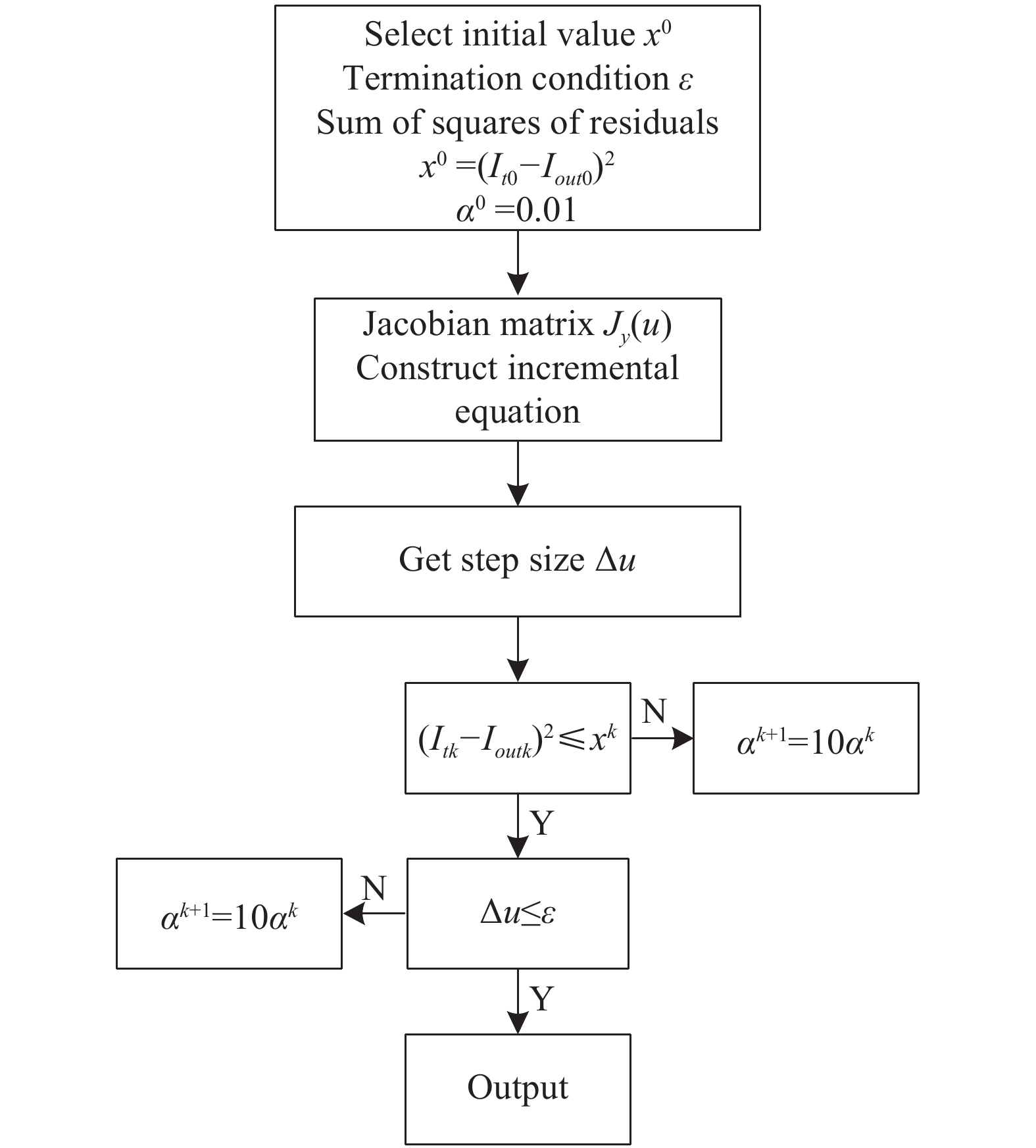
LM算法的求解步骤如图2所示。
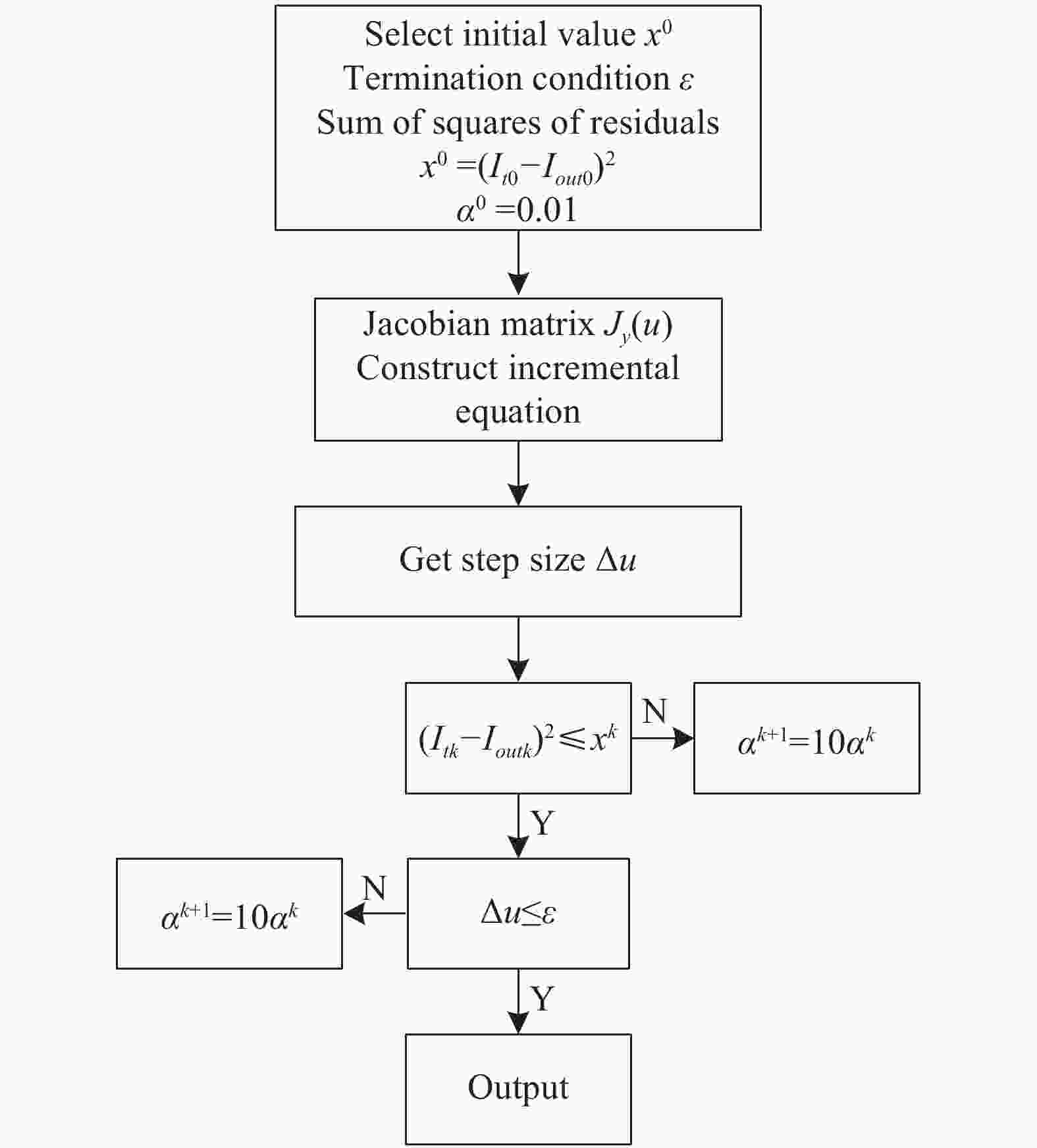
图 2 LM算法流程图
Figure 2. Flow chart of LM algorithm
求出系统参数后,代入放置样品的光强公式,并进行向量化算子运算。此时系统中的未知参数为样品Mueller矩阵的16个元素,通过拟合法求出样品的矩阵,并与实测矩阵作对比,验证LM算法的有效性并进行分析。
-
为了给系统光学元件参数进行精密定标,需要解出元件参数值。实验中定标的参数为起偏器和检偏器方位角,两个角速度为1:5的匀速旋转的1/4波片的初始方位角和相位延迟。设计了如下实验步骤:
(1):调整测量参数,在样品台发放置标称值(24.90±0.30) nm的SiO2/Si标准样片,两旋转波片分别以1:5的角速度匀速旋转。在波长500~900 nm范围内采集81组光强,根据公式求出公式(6)和公式(7)进行拟合。此时待拟合参数中不含样品Muller矩阵;
(2):放置标称值(91.21±0.36) nm的SiO2/Si标准样片,以同样的步长n在一个周期内采集光强,共采集(360º/n1
)*(360º/n2)组。把步骤一中解出的参数和出射光强、入射光强代入方程公式; (3):根据薄膜样品的层数和基底材料的光学特性,用传输矩阵法建立与样品光学常数、样品厚度和入射角的穆勒矩阵,用最小二乘法解出样品的Mueller矩阵及膜厚参数。实验流程图如图3所示。
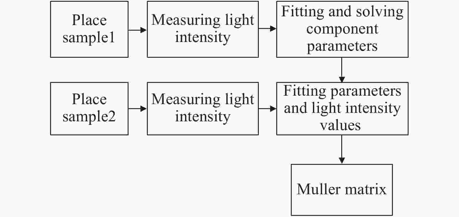
图 3 实验流程图
Figure 3. Flow chart of experiment
-
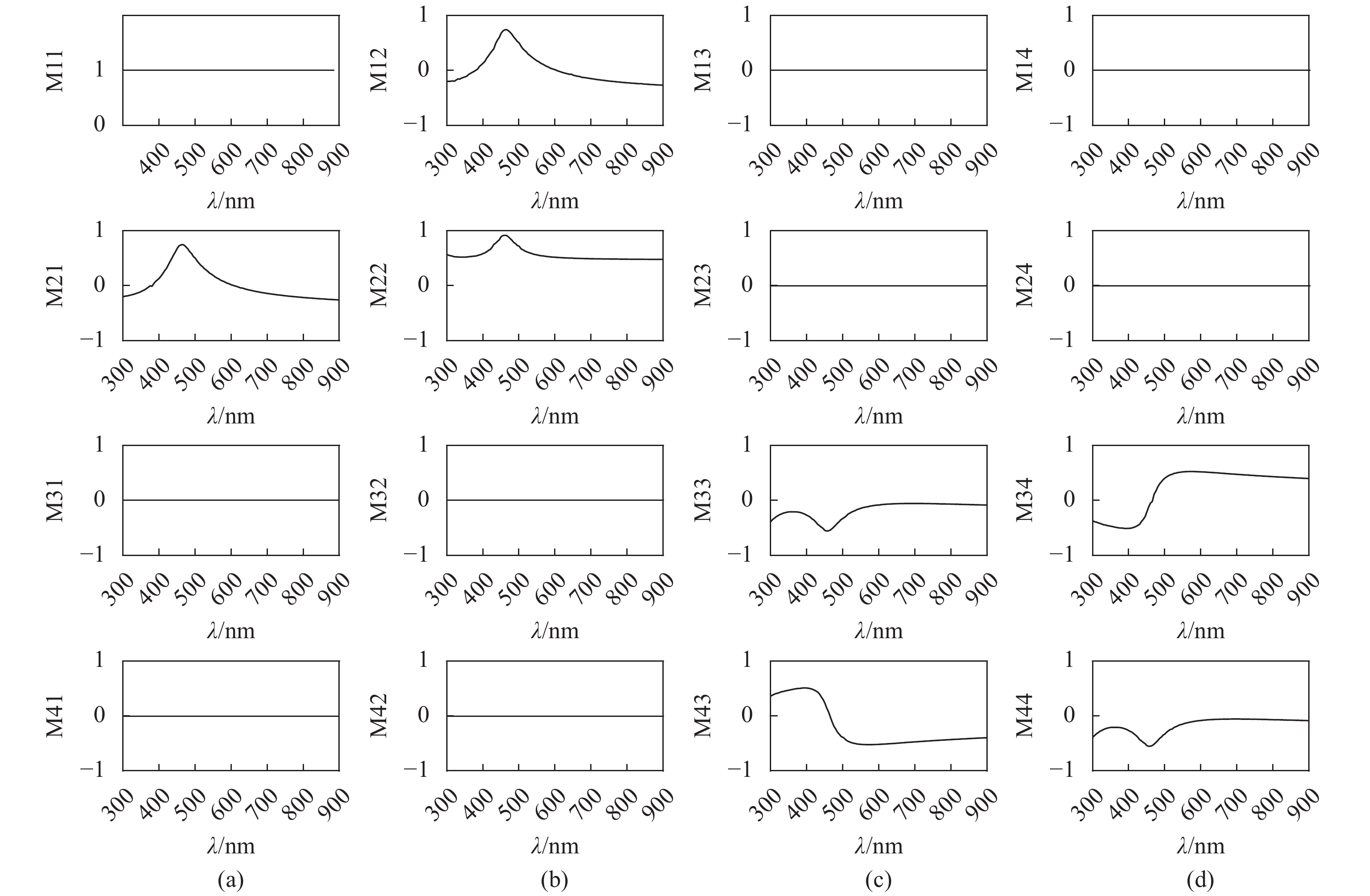
选用已知光学常数(Ψ,Δ),标称值为25 nm,标定值为(24.9±0.3) nm的SiO2/Si标准样片,测量出射光强放入方程迭代。根据各向同性薄膜的传输特性,建立样品的穆勒传输矩阵,图4为穆勒矩阵光谱图。

图 4 25 nm SiO2/Si标准样片穆勒光谱图
Figure 4. Mueller spectrum of 25 nm SiO2/Si film thick sample
图4中的M11是包含光强信息的矩阵元,为了消除光强值的影响,M12~M44的曲线是对M11矩阵元做穆勒矩阵归一化处理后的样品光学常数随波长的变化曲线。波长在500~900 nm范围内,样品的Mueller矩阵光谱图比较稳定。起偏器和检偏器的旋转周期分别以400 ran/min和80 ran/min的角速度匀速旋转,用100 W高精度钨卤素灯作为光源,在一个周期0.75 s内,共采集81组数据。设定收敛值小于0.30,迭代到60次时停止迭代。用LM法进行拟合,迭代曲线如图5所示。
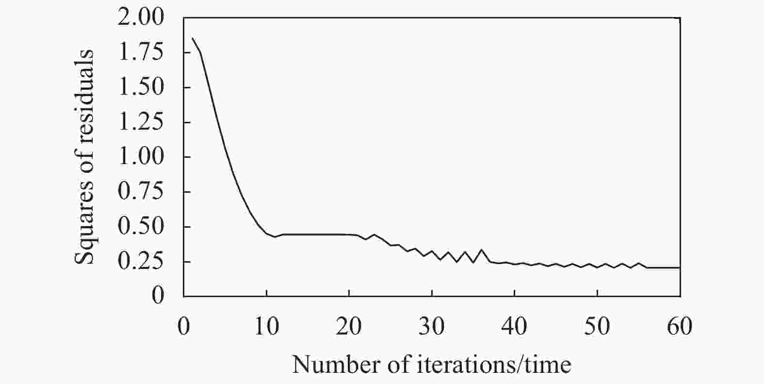
图 5 残差平方和迭代图
Figure 5. Residual sum of squares iteration
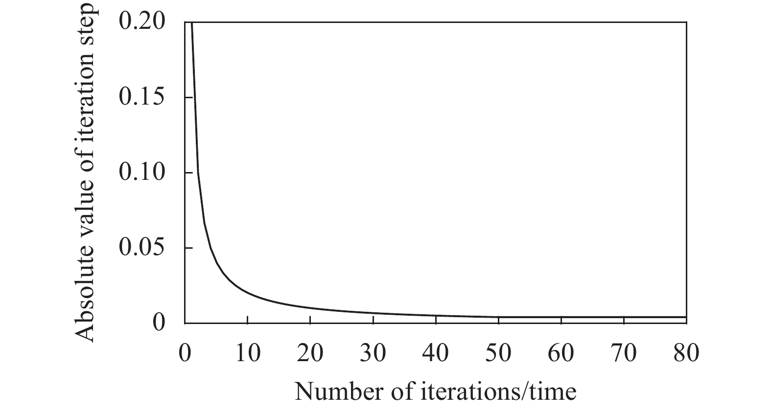
从计算光强值与测量光强值残差平方和的迭代曲线可以看出,经过10次迭代,步长的减小趋势已逐渐缓慢,参数已靠近精确值,接着不断缩短步长。当迭代到50次之后,步长绝对值和残差平方和达到最小值,此时关于参数的雅可比矩阵为零矩阵。之后残差平方和以固定步长0.005正反方向交互震荡,取最小值0.24,如图6所示。可以看出,用LM算法进行迭代,不仅收敛速度快,在较短的时间内计算出精确值,同时不断调整步长情况下,可以避免使计算结果陷入局部最优解的情况。表1中为系统参数的拟合结果。

图 6 步长绝对值变化图
Figure 6. Change diagram of step absolute value
表 1 元件各参数计算值
Table 1. Calculated values of various parameters of components
Component Parameter Value/(º) Polarizer Orientation A 44.787 5 Waveplate C1 Orientation c1 0.111 5 Waveplate C1 Retardation Δ1 97.242 5 Waveplate C2 Orientation c2 –0.108 6 Waveplate C2 Retardation Δ2 97.242 5 Analyzer Orientation P –44.979 1 -
为了验证拟合参数的准确度,需要将表1中的参数值进行仿真模拟。在仿真计算前,将薄膜的膜层结构等效为理想模型,建立光学常数和厚度的柯西模型,得到薄膜的穆勒矩阵。选用标称值为90 nm,标定值为(91.21±0.36) nm的SiO2/Si标准样片对定标参数进行验证,每隔9.375 ms采集一个光强数据,共采集81组数据。建立光强关于样品穆勒矩阵的非线性最小二乘模型,并用LM算法进行迭代,样品的穆勒矩阵随波长变化的仿真图如图7所示。
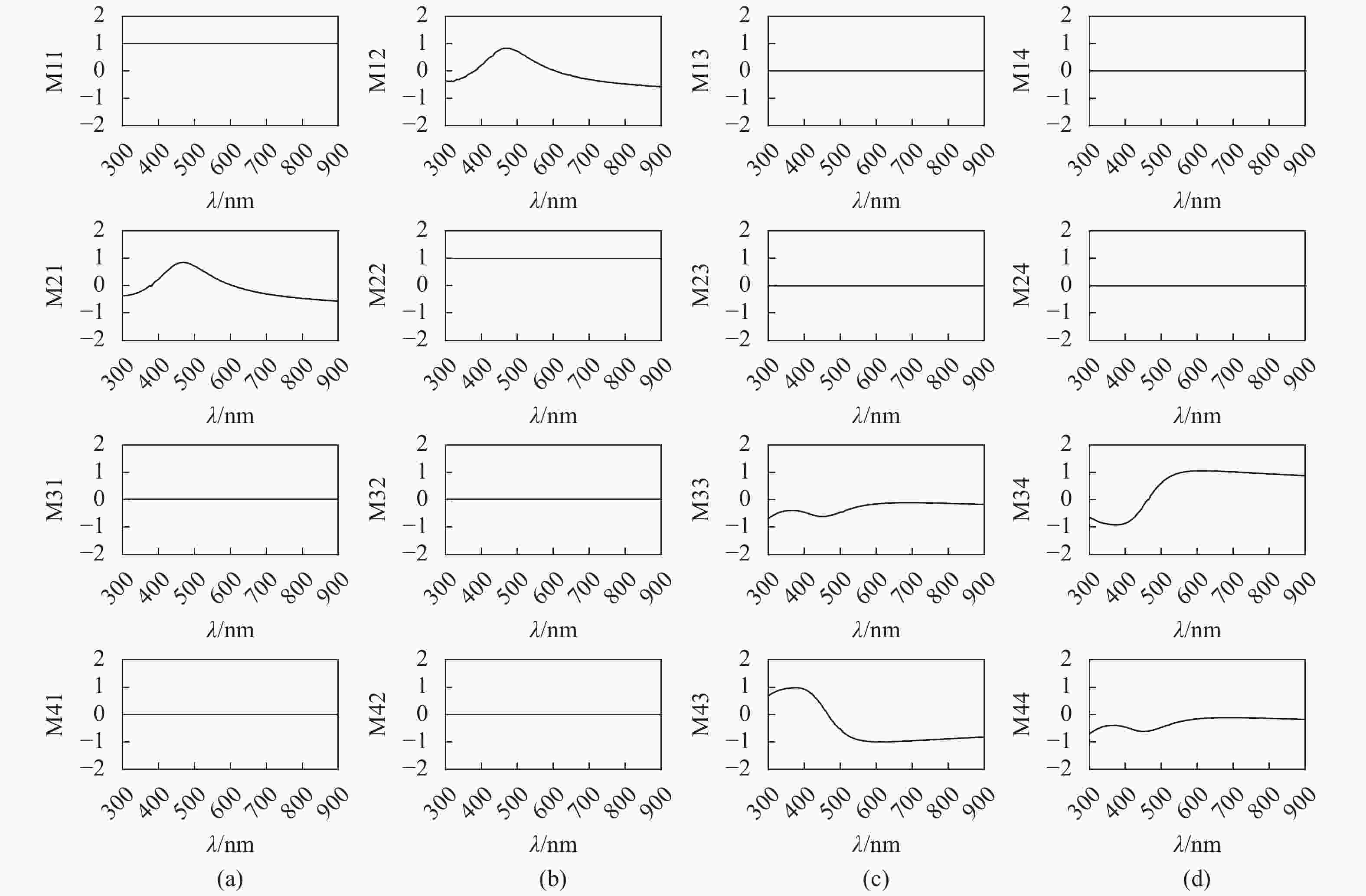
图 7 91 nm SiO2/Si标准样片穆勒光谱图
Figure 7. Mueller spectrum of 91 nm SiO2/Si standard sample
图7模拟了样品用LM算法计算的穆勒光谱矩阵元素法变化,与样品的定标穆勒矩阵相比所有元素的相对误差最大为0.36%。在波长在300~500 nm范围内,误差相对较大,证明系统信噪比较高。波长大于500 nm时,光谱曲线逐渐趋于稳定,用此段穆勒矩阵光谱数据分析,得到样品的厚度计算值为91.53 nm,相对误差为0.35%,证明表1中的参数计算值符合系统的实际参数值,验证了LM算法在椭偏系统定标中的可行性。
单一的膜厚测量误差无法体现LM算法的优越性,同时用多点定标法测量了系统81组偏振态的传输矩阵X,则样品的穆勒矩阵如公式(18)所示:
$$ {M_{{\text{样品}}}}{\rm{ = }}M_{{C_2}}^{{\rm{ - }}1}M_P^{{\rm{ - }}1}{E^{{\rm{ - }}1}}XM_A^{{\rm{ - }}1}M_{{C_1}}^{ - 1} $$ (18) 实验中的81组偏振态用多点定标法确定系统的传输矩阵X,将拟合参数和标准样片的穆勒矩阵作为已知量带入,反演出各偏振态的出射斯托克斯矢量,与实测光强的残差平方和如图8所示。
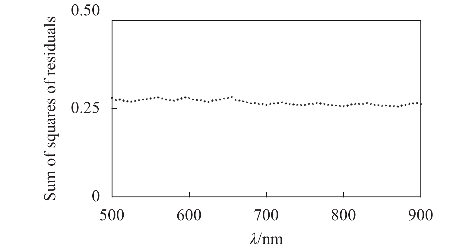
图 8 光强残差平方和变化点状图
Figure 8. Spot chart of the change of the sum of squares of light intensity residuals
由图8可以看出,在波长500~900 nm范围内,用多点定标法获得的归一化光强的残差平方和约在0.25~0.28之间。而LM算法迭代的收敛值精确到0.24,高于传统多点定标法1%,说明了此算法的可行性与高精度。
-
在表征方法中,偏振片的透光轴方位角、1/4波片的初始方位角和相位延迟是拟合方程通过LM算法迭代直接求解的,不存在误差,系统主要存在退偏产生的误差。理想情况下,起偏器的偏振度为1,但实际过程中并不能制造标准的偏振片,导致出射光不是完全的线偏振光。而计算得到的穆勒矩阵是完美非退偏矩阵,从而产生退偏误差。
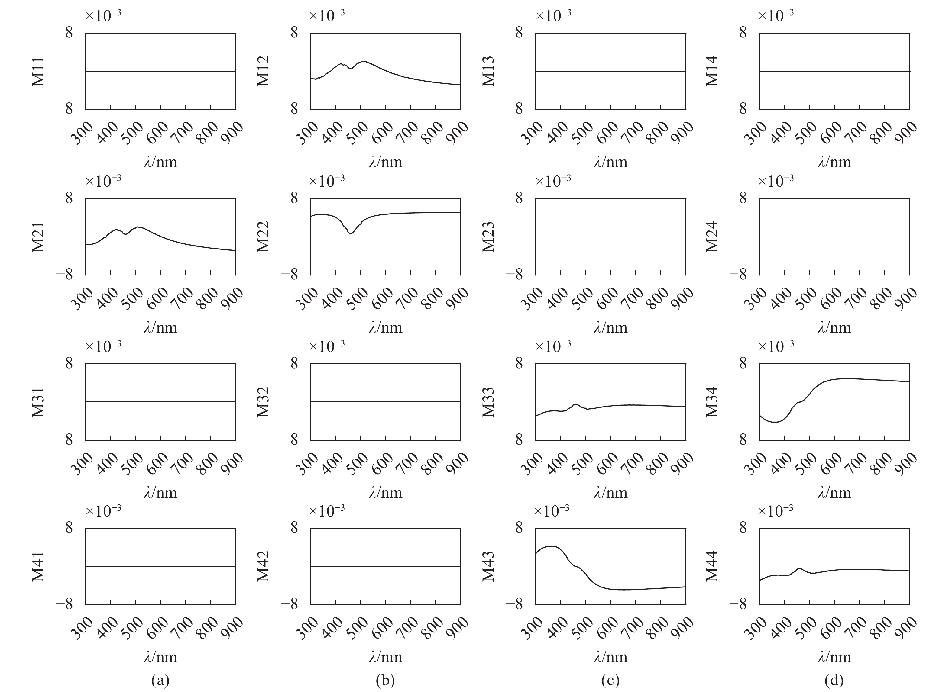
图9为样品考虑退偏的穆勒矩阵光谱图,图中曲线走向与计算穆勒矩阵光谱图基本相同,表明退偏误差对定标结果不会造成明显的影响。图10为退偏误差矩阵ΔM,图中可见在400~500 nm波长范围内,各元素的误差达到最小值;当波长大于600 nm,误差趋于稳定。穆勒元素的相对误差都在0.008单位内,远小于穆勒元素的数量,表明当定标系统光学元件参数时,退偏误差可以忽略。
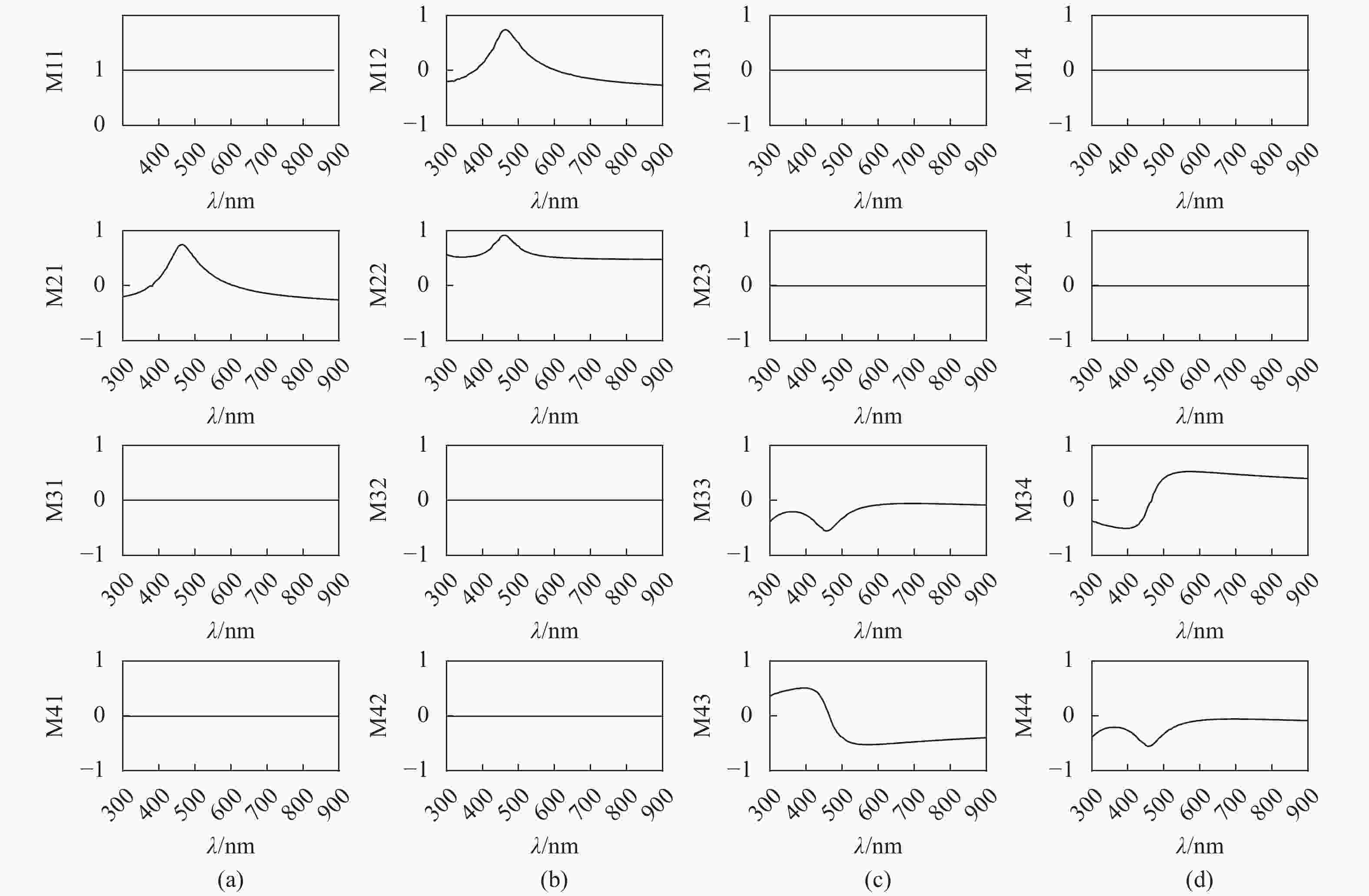
图 9 91 nm SiO2/Si标准样片含退偏穆勒光谱图
Figure 9. Mueller spectrum with depolarization of 91 nm SiO2/Si standard sample

图 10 91 nm SiO2/Si标准样片误差矩阵光谱图
Figure 10. Error matrix spectrum of 91 nm SiO2/Si standard sample
-
文中采用非线性最小二乘拟合法建立等效模型光学常数和膜厚的穆勒矩阵模型,得到偏振光的传输模型,实现对双旋转穆勒椭偏参数的标定。通过标定值(24.90±0.20) nm的SiO2/Si标准样片的测量出射光强,用LM算法对目标函数进行迭代,求出测量系统的偏振元件参数。再通过测量标定值(91.21±0.36) nm的SiO2/Si标准样片进行仿真计算。分析穆勒光谱图得膜厚的计算值为91.53 nm,相对误差为0.35%,验证了拟合参数的有效性,并与传统的多点定标法相比较,说明了LM算法在穆勒测量系统参数定标中,是一种能准确找到全局最优解、收敛速度快、测量精度高的表征方法。
Study on LM algorithm in Mueller's ellipsometry calibration method
-
摘要: 依据穆勒椭偏测量方法中偏振光的传输方式,提出了一种椭偏系统中光学元件参数的定标方法。通过建立出射光强关于起偏器和检偏器透光轴方位角、旋转补偿器方位角和相位延迟的非线性最小二乘模型,用列文伯格−马夸尔特(Levenberg-Marquardt,LM)算法对初始参数进行迭代。求解出光学元件参数的精确值,从而实现对元件的定标。通过仿真实验,利用已知穆勒(Mueller)矩阵且标定值为(24.90±0.30) nm的SiO2/Si标准样片,基于LM算法迭代计算光强值的残差平方和。实验可得当迭代次数为50次时,残差平方和收敛到最小值0.24;与传统多点标定法进行对比试验,验证了基于LM算法求解光学参数的可行性;用标定值为(91.21±0.36) nm的SiO2/Si标准样片进行验证,得到膜厚的计算值为91.53 nm,相对误差为0.35%。结果表明:在穆勒椭偏系统参数标定中,LM算法具有收敛速度快,计算精度高等优点。Abstract: According to the transmission method of polarized light in Mueller ellipsometry method, this paper presented a method for calibrating the optical element parameters in ellipsometry system. By establishing a nonlinear least squares model of outgoing light intensity with respect to orientations of transmission axis of the polarizer and analyzer and orientations and retardation of the rotation compensator, the initial parameters were iterated with Levenberg-Marquardt (LM) algorithm. Accurate values of optical element parameters could be obtained, so as to achieve the calibration of components. Through the simulation experiment, using the SiO2/Si standard sample with the known Mueller matrix and the calibration value of (24.90 ± 0.30) nm, the residual square sum of the light intensity value was calculated based on LM algorithm. When numbers of iterations accumulate to 50, the sum of squares converges of the residuals of the measurement and calculation was limited to 0.24. Then compared with the traditional multi-point calibration method, the feasibility of solving optical parameters based on LM algorithm was verified. Fitting results were validated by SiO2/Si standard sample with calibration value of (91.21±0.36) nm. Calculated film thickness was 91.53 nm and the relative error is 0.35%. Results proved that LM algorithm has advantages of rapidly converging and high precision in the parameter calibration of the Mueller ellipsometry system.
-
Key words:
- parameter calibration /
- Mueller matrix /
- ellipsometry /
- LM algorithm /
- standard sample
-
图 4 25 nm SiO2/Si标准样片穆勒光谱图
Figure 4. Mueller spectrum of 25 nm SiO2/Si film thick sample
图 7 91 nm SiO2/Si标准样片穆勒光谱图
Figure 7. Mueller spectrum of 91 nm SiO2/Si standard sample
图 8 光强残差平方和变化点状图
Figure 8. Spot chart of the change of the sum of squares of light intensity residuals
图 9 91 nm SiO2/Si标准样片含退偏穆勒光谱图
Figure 9. Mueller spectrum with depolarization of 91 nm SiO2/Si standard sample
图 10 91 nm SiO2/Si标准样片误差矩阵光谱图
Figure 10. Error matrix spectrum of 91 nm SiO2/Si standard sample
表 1 元件各参数计算值
Table 1. Calculated values of various parameters of components
Component Parameter Value/(º) Polarizer Orientation A 44.787 5 Waveplate C1 Orientation c1 0.111 5 Waveplate C1 Retardation Δ1 97.242 5 Waveplate C2 Orientation c2 –0.108 6 Waveplate C2 Retardation Δ2 97.242 5 Analyzer Orientation P –44.979 1  下载: 导出CSV
-
[1] Liu Ninglin. Research on mid-infrared mull-er matrix spectroscopic ellipsometer[D]. Huazhong: Huazhong University of Science and Technology, 2019. (in Chinese) [2] Wu Suyong, Long Xingwu, Yang Kaiyong. An error processing technique for ellipsometry measurement system which minimizes the error of optical parameter characterization of thin films [J]. Acta Optica Sinica, 2012, 32(6): 280. (in Chinese) [3] Fan Zhentao. Research on the advanced parameters problem of muller matrix ellipsometry system[D]. Beijing: University of Chinese Academy of Sciences , 2019. (in Chinese) [4] Li W, Zhang C, Jiang H, et al. Depolarization artifacts in dual rotating compensator Mueller matrix ellipsometry [J]. Journal of Optics, 2016, 18(5): 055701. doi: 10.1088/2040-8978/18/5/055701 [5] Liu S Y, Chen X G, Zhang C W. Development of a broadband Mueller matrix ellipsometer as a powerful tool for nano structure metrology [J]. Thin Solid Films, 2015, 584(1): 176-185. [6] Dai Lina, Deng Jianxun, Wang Juan, et al. The optical constants and Euler angles of anisotropic thin films were studied by using a single wavelength ellipsometer [J]. Journal of South China Normal University (Natural Science Edition), 2019, 51(4): 14-20. (in Chinese) [7] Zhen Tang. Mul-tipoint calibration method based on stok-es ellipsometry measurement system [J]. Chinese Journal of Lasers, 2012, 39(11): 163-167. (in Chinese) [8] Urban F K I, Barton D. Numerical ellipsometry: Use of parameter sensitivity to guide measurement selection for transparent anisotropic films [J]. Thin Solid Films, 2018, 663(10): 116-125. [9] Meng Fanxue. A hybrid algorithm for solving nonlinear least squares problems[D]. Shanghai: Shanghai Jiao Tong University, 2011. (in Chinese) [10] Yang Liu, Chen Yanping. A new globally con-vergent levenberg-marquardt method for sovling nonlinear system of equations [J]. Mathematica Numerica Sinica, 2008, 30(4): 388-396. (in Chinese) [11] Zhang Ruizhi, Luo Jinsheng, Chen Minlin. Calibr-ation method for azimuth angle of a rotary polarizer-type automatic ellipsometer polarizer-type [J]. Journal of Applied Optics, 1988(6): 36-39,73. (in Chinese) [12] Azzam R M A, Lopez Ali G. Accuratecalibration of the four-detector photopola-rimeter with imperfect polarizing optical elements [J]. Journal of the Optical Society of America A, 1989, 6(6): 1513-1521. [13] Krishnan S. Calibration, properties, and applications of the division-of-amplitude photopolarimeter at 632.8 and 1523 nm [J]. Journal of the Optical Society of America A, 1992, 9(9): 001615. doi: 10.1364/JOSAA.9.001615 [14] Azzam R M A, Masetti E, Elminyawi I M, et al. Construction, calibration, and testing of a four etector photopolarimeter [J]. Review of Scientific Instruments, 1988, 59(1): 84-88. doi: 10.1063/1.1139971 [15] Azzam R M A. Arrangement of four photodetectors for measuring the state of polarization of light [J]. Optics Letters, 1985, 10(7): 309-311. doi: 10.1364/OL.10.000309 [16] Liao Yanbiao. Polarization of Optics[M]. Beijing: Science Press, 2003. (in Chinese) -

 点击查看大图
计量
- 文章访问数: 481
- HTML全文浏览量: 180
- PDF下载量: 37
- 被引次数: 0


