Networking method of multi-view stereo-vision measurement network

机器视觉测量技术通过单个视点相机只能得到待测物的部分信息，难以满足观测需要。多视点立体视觉测量网络在三维重建中表现良好，能够满足高精度和密集型测量场合的需要^[1]。该测量网络在待测物周围不同位置布置观测相机（或利用单摄像机多站位移动拍摄），然后拍摄待测物各角度图像，进行参数标定、特征匹配等图像信息处理，最后通过三维重建^[2-3]实现待测物三维信息的获取。

针对多视觉组网三维测量，国内外的机构和学者进行了深入而广泛的研究。Mason率先研发出了CONSENS系统，该系统基于专家知识，将待测物模型转换成基本几何基元，然后利用四台相机的测量组网对每个平面成像^[4]；继Mason的研究之后，Olague开发了EPOCA系统，该系统能够自动为测量系统设计一个合适的测量组网。Olague与Chen及Li忽略了与距离相干的约束条件，仅考虑采用最小化函数的视场模型，基于相机景深及遮挡区域设置可见性约束函数等方式破解该测量难题，但测量方案的精确性并不高^[5-6]。Alsadik考虑了可见性约束条件、覆盖率，对测量相机做了分类和筛选过程，再利用惩罚函数不断优化筛选，得出最优的视觉测量网络^[7]。该测量网络在遮挡区域和观测精确度的影响上未做考虑，不具有完备的普适性。国内，于起峰和姜广文等人研究船体变形的测量难题，提出了一种视觉测量组网方法，先定义基准并布置多个相机间的位姿，然后设置了各相机视点和定义基准之间数学物理模型，最后通过相机视点来估计定义基准与待测物间的位姿和变形量^[8]。在测量网络的优化上，哈尔滨理工大学乔玉晶等人研究了一种多视觉测量组网规划策略，该策略基于遗传算法，以测量网络的覆盖率与待测点云的三维不确定度为验证指标，综合考虑观测的约束条件，不断对测量组网进行优化，优化趋于稳定即得到最优组网，最后通过测量实验证实了组网策略的可行性^[9]。上述视觉组网均汇聚在分析测量视点的约束条件，包括可见性约束、景深约束、视场约束及分辨率等，而所有这些技术都需要一个良好的初始网络专家（即先验知识）。但仅凭经验而无理论支撑的布置相机网络无法保证测量的全覆盖和精确性，因此多视点立体视觉测量方法要综合考虑待测物模型的定义、视点相机的位姿布置、观测约束条件等因素，设计出测量网络，满足全覆盖和高精度的要求。

综上所述，文中提出了一种多视点立体视觉测量网络组网的优化方法，实现最佳多视觉传感网络布局。通过获得待测物模型，生成初始候选视点位姿，然后根据可视化约束条件对视点进行迭代筛选，设定了覆盖率和精确度来保证立体视觉测量网络的可行性，最后优化出需要最少数量相机的最优多视点测量网络。

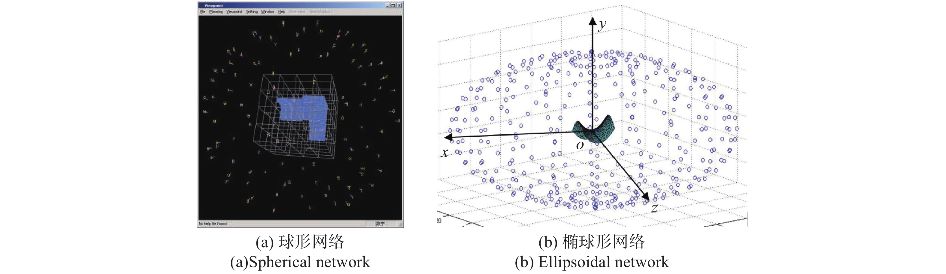
为了使用立体视觉测量网络获取待测物的三维信息，并结合测量精度、覆盖率以及最少相机数的要求，来考虑立体视觉测量网络的所有可能的约束条件，找到合适的相机成像位姿。为简化初始网络几何模型，Chen和Li等采用网络几何模型为球形^[6]，如图1(a)所示，由于球形网络中的测量节点距离被测物中心半径相等，这种球形网络几何模型没有考虑被测物本身的几何形状，在不同方向上其尺寸不同，所以文中设计了多视觉测量网络初始几何模型为椭球模型，并以马鞍模型为例，其初始化测量网络如图1(b)所示，图中的圆圈代表视觉传感器所处的测量网络节点的位置。

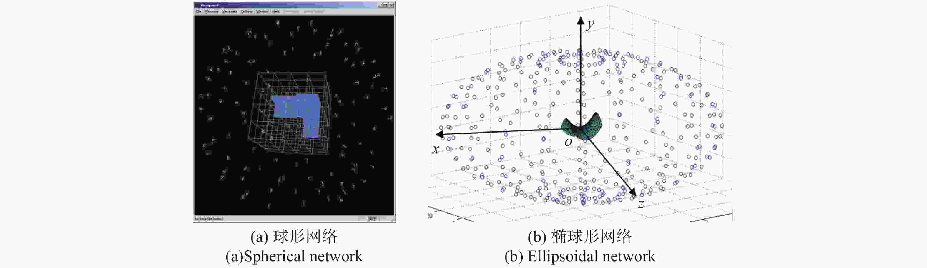
Figure 1.  Visual measurement network model

图中将被测物模型中心定义为三维坐标系原点；x轴的正方向：从三维坐标系原点指向距离原点最远的点，大小为两点之间的距离，定义为椭球体的第一个赤道半径,记为a；y轴正方向：过原点作x轴的垂线，指向距离原点最远的点，大小为两点之间的距离，定义为椭球体的第二个赤道半径，记为b；z轴的正方向遵循空间向量的右手定则，定义极半径c为物点距离xoy平面的最远距离。

相机光轴垂直于待测物感兴趣区域时能够得到清晰图像，同时三维重构过程中所涉及的覆盖率和重构精度与相机位置及其他限制条件有关。在设定坐标系和拟合的椭球体模型后，视点距离待测物最远${D_{\max }}$和最近${D_{\min }}$的可能距离可以计算为：

式中：i=camera1、camera2、camera3、…。其他限制条件参数：相片大小、分辨率、视场的计算过程如表1所示。

要达到较高的覆盖率需要将相机放置与待测物的最远距离，但此处测量得到的点云精度低；保证精度较高的点云数据需要将相机放置与待测物的最近距离，但此时覆盖率又会降低。实验表明，将相机布置在最远与最近距离的平均值处可以获得最佳的成像效果，故取二者的平均值作为视点分布最佳距离估计${D_{\rm{optimum}}}$^[10]，如公式（3）所示：

合理的视点位姿将使立体视觉测量网络能够精准的测量待测物的点云数据。结合相机姿态参数、被测物点云的椭球体参数($ a,b,c$)和最佳距离估计，对视点位姿的布置分以下三步进行：(1) 根据椭球体坐标系定位视点分布的基线中心；(2) 在基线中心布置视点相机；(3) 为每一个布置的相机设定位姿。据椭球体设置的基线中心计算公式（4）所示：

式中：${X_i}$${Y_i}$${Z_i}$表示各视点的基线中心坐标，轨道角计算如下：${\alpha _i} = {\alpha _{i - 1}} + \Delta \alpha $，${\beta _i} = {\beta _{i - 1}} + \Delta \beta $，每一个轨道角$\Delta \alpha $、$\Delta \beta $都有一个基线坐标，基线坐标要综合相机视点距离、视点之间的重叠区域，然后在初始已知视点位姿的基础上进一步获取每个视点在基准坐标系的位姿。该方法将每个视点相机的光轴设置为朝向基准坐标系原点，即椭球体的中心位置O。若待测物形状严重不规则，可以适当改变光轴朝向，能够使每个视点尽可能覆盖更大观测区域为宜。相机位姿布置如图2所示，为直观显示，仅布置了椭球体赤道一周。

Figure 2.  Camera position layout diagram

通过SFM技术获取的待测物点云，由于实验光线不佳以及特征匹配不准等因素会出现离群点，需要对点云数据进行去噪滤波。该方法采用统计学的方法，计算每个点到相邻点距离的均值，该值不在设定区间内则为离群点，予以剔除，进一步提高点云数据的准确性。

经初始化的每个相机要测试可以覆盖哪些点，该方法将生成的点云中相邻三个点进行连线，构成三角区域，然后计算出每个三角区域的法向量，再通过各三角区的法向量计算相机对三角平面的可见性，最终确定每个相机对每个点的可见性。马鞍模型的三角区的法向量示例如图3所示。

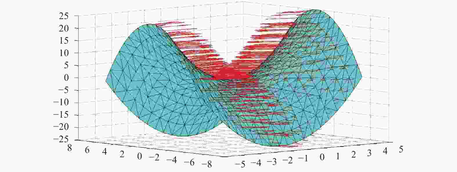
Figure 3.  Schematic diagram of the normal vector of the triangle

在使用SfM技术获得待测物的三角网格模型验证每个点的可见性之后，需要考虑可视化约束条件，来优化椭球模型初始立体视觉测量网络。该方法主要考虑的约束条件有可见性约束、入射角约束和视场约束，具体约束条件的表述形式参见参考文献[9]。

文中研究的目的是在最佳立体视觉测量网络中找到最小的相机数目，既保证覆盖范围又保证高精度。将椭球体模型表面布局好的视觉传感器依据覆盖率分为冗余相机和非冗余相机^[6]，并通过循环迭代逐步过滤掉冗余相机，达到相机最少的目的。

视点的迭代筛选详细步骤如下：

（1）总结归纳相机规划问题的影响因素，使用运动恢复软件（Visual SFM）获取稠密的待测物点云数据，确定相机的可见性约束条件；

（2）根据可见性约束条件，通过MeshLab软件在待测物点云中生成三角区域，计算法向量，验证相机对三角平面的可见性，进一步得出相机对每个点的可见性；

（3）通过相机对点的可见性，将相机进行聚类分析，对点云中每个点进行划分，分为全覆盖点和过覆盖点。实验表明，三个相机已能够完整覆盖一个点，因此将同时出现在三个相机中的点定义为全覆盖点，出现在多于三个相机中的点定义为过覆盖点；依据覆盖点对相机进行分类，观测到全覆盖点的相机定义为合理相机，观测到过覆盖点的相机定义为冗余相机，若同时观测到全覆盖点和过覆盖点仍定义为合理相机；

（4）对上述分类相机作统计，按照相机的覆盖率排序，删除覆盖率低的冗余相机，持续更新测量组网。重复步骤（2）、（3）、（4），直到没有冗余相机；

（5）最终待测物点云的所有点均有且仅有三个相机覆盖，停止更新相机网络。

经过迭代筛选后的相机视点马鞍仿真分布如图4所示。

Figure 4.  Viewpoint simulation result distribution diagram

该测量实验以灯罩为测量对象，基于张正友标定法进行相机标定，对比已有方法球形测量网络，将优化后所需相机数目、观测覆盖率和测量精度作为评估指标，验证该方法的可行性。相机数目和覆盖率均可直接获得，精度可利用光束法平差计算优化所得到的点云的均方根误差判定。

为降低试验成本，该实验利用Motoman机械臂夹持单摄像机多站位移动拍摄，为保持在待测物周围不同位置布置观测相机的测量方式精度一致，在每个站位点均需要进行一次标定，实验以如图5所示的灯罩为测量实验对象，将灯罩圆周表面按照英文字母A-K标记一周，两个标记点间隔四个空格。首先使用SFM技术获取灯罩的点云数据，获取点云共包括6 800个待测物点，并生成椭球体初始测量网络，如图6所示。再使用Meshlab软件生成灯罩点云数据的三角区域，计算法向量，验证相机对每个点的可见性。

Figure 5.  Experimental platform and real shot

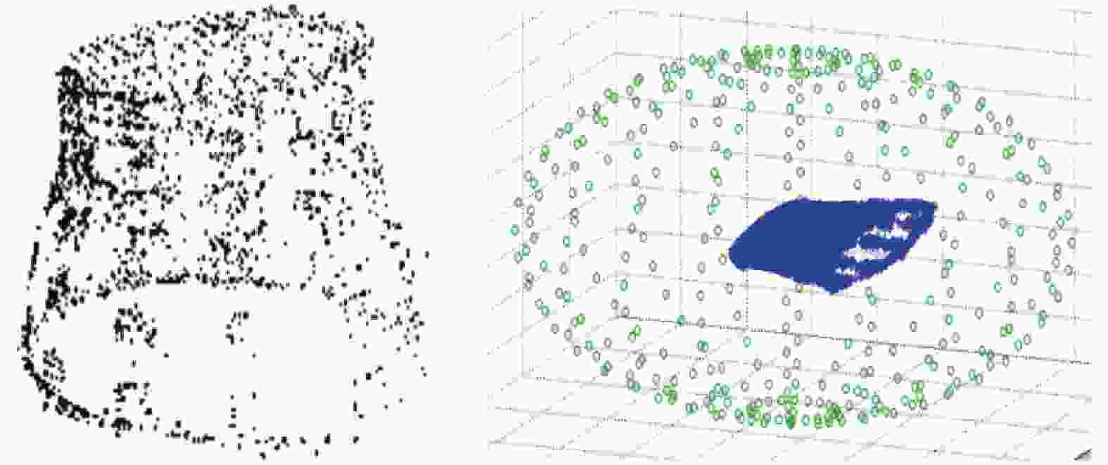
Figure 6.  Shade point cloud and ellipsoid initial measurement network

立体视觉测量组网实验中使用的相机型号为大恒${\rm{MER - 130 - 30UM}}$，相机焦距为$3.5\;{\rm{mm}}$，拍摄分辨率为$1\;280\;({\rm{H}}) \times 1\;024\;({\rm{V}})$，像素尺寸大小为5.2 μm × 5.2 μm。

该实验对椭球测量网络和球形测量网络中的相机（即大恒${\rm{MER - 130 - 30UM}}$）进行标定，固定标定板，确保实验过程中位置不会变动，在每个视点位姿下各采集10幅标定板图像，方便挑选。图7仅给出一组经挑选后三个视点位置拍摄的图像。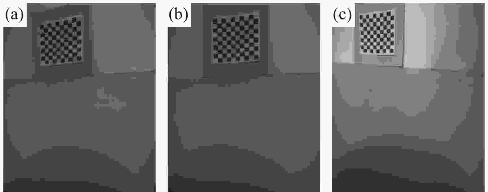

Figure 7.  Image of three viewpoint positions

由于实验光线、噪声等不良条件的作用，需要对标定图像预处理。在Windows系统上通过Matlab软件对图像进行去噪滤波，再进行角点检测，最终得到观测相机的内外参数。文中以光圈f/2.8相机测量为例，给出了椭球体测量网络四个相机的内外参数，如表2所示。

根据上文标定结果，实验中相机的理论值与实际值大致相差1 pixel，通过光束法平差，据标定结果得到的相机内外参数来计算理论物方坐标，再与真实物方坐标进行运算，得出两坐标的均方根误差。

文中采用控制变量法，对比该方法优化下的椭球形测量网络和已有方法球形测量网络，在椭球形测量网络和球形测量网络中使用同一型号的大恒MER-130-30UM相机。依据上述参数和公式(1)~(3)分别计算出测量视点的三个距离：

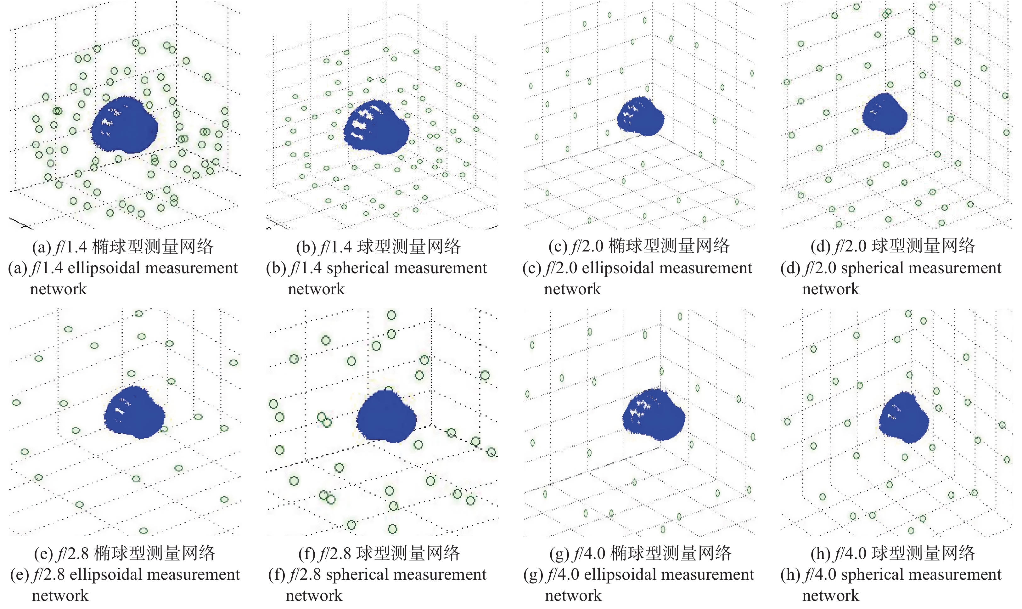
在椭球形测量网络中，椭球体的两个赤道半径和极半径分别为a = 136 mm，b = 105 mm，c = 101 mm；而在球形测量网络中，各半径相等即a = b = c = 136 mm。相机成像受景深影响较大，故视觉测量网络会受较大影响，而景深主要受光圈、镜头焦距、与拍摄物的距离三个要素的影响，此次实验中焦距和距离不变，故只考虑光圈的影响。实验设置了不同光圈（景深）下灯罩在椭球形测量网络和球形测量网络中成像效果对比，如图8所示。

由图8可知，椭球形和球形测量网络在不同光圈（景深）下，经过该方法迭代筛选后相机数目均会明显减少，并且椭球形测量网络在各光圈（景深）下都比球形网络需要更少的相机数目。在此次实验中，在光圈f/2.8后，两测量网络下的相机数目均趋于稳定，椭球形网络需要22台相机，球形网络需要30台相机，即测量效率提高了26.7%。在光圈f/2.0下，观测效率虽提升到了28%，但是仍需要较多相机，且未趋于稳定，故不做选择。测量网络相机数目对比如表3所示。

Figure 8.  Measurement network for aperture f/1.4,f/2.0,f/2.8,f/4.0

将特征点均匀地贴在待测物表面，总数记为${w_{\rm{all}}}$，通过迭代筛选后立体视觉测量组网来观测特征点数目来反映组网的覆盖率。利用相机筛选的方法，若一个特征点同时被组网中的三个相机拍摄，标记该特征点，记录总数为${w_{\rm{visual}}}$，覆盖率记为$p$，那么覆盖率即为标记特征点数和总特征点数的商，如公式（5）所示：

覆盖率实验仍然设置了不同光圈（景深）下灯罩表面特征点在优化后的椭球形测量网络和球形测量网络对比，如图9所示。在光圈f/2.8后，两测量网络均达到了100%的全覆盖率，在f/1.4、f/2.0虽未全覆盖，但椭球形网络仍具有比球形网络更高的覆盖率。

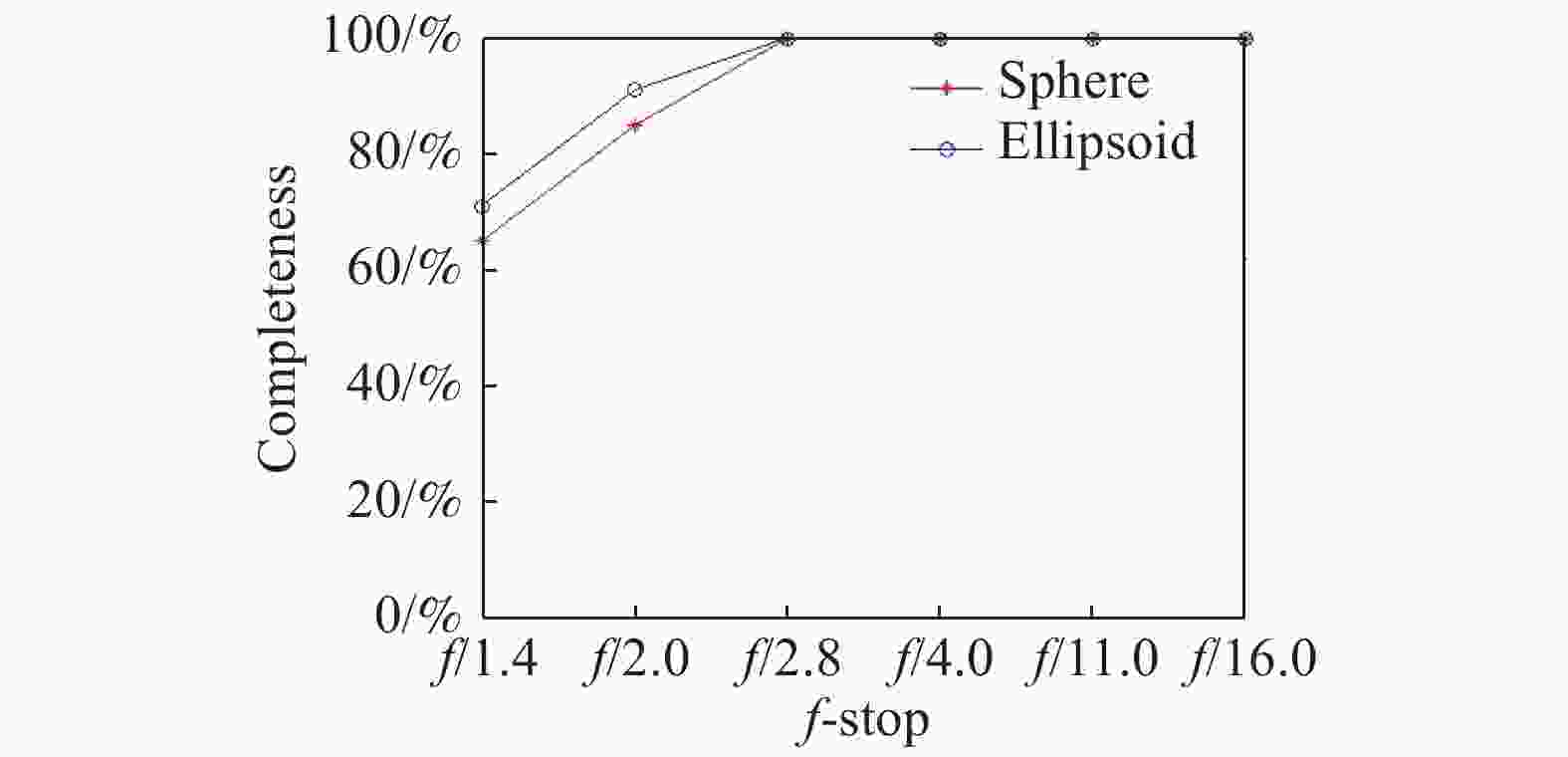
Figure 9.  Coverage comparison chart

为了评估优化后立体视觉测量网络的测量精确度，采用光束法平差的整体算法，计算点云的协方差矩阵${Q_{XX}}$，如公式（6）所示：

式中：$A$是协方差中的设计矩阵；$P$是点云观测值的权值；$\sigma _0^2$是单位权值。该实验中已知相机拍摄的外方位元素$\left( {{{{X}}_S},{{{Y}}_S},{{{Z}}_S},\omega ,\phi ,\kappa } \right)$和像点坐标$(x,y)$，仅物方点坐标为待求值。据$\left( {{{{X}}_S},{{{Y}}_S},{{{Z}}_S},\omega ,\phi ,\kappa } \right)$和$(x,y)$即可求得相对于物方点坐标的传播误差。

精度分析实验设置在不同光圈（景深）下对椭球形测量网络和球形测量网络的数据对比，如表4所示（数据单位为mm）。数据表明，在不同景深下，椭球形网络相比球型网络测量精度均有明显提升，主要原因在于球形网络中一些相机未能处于观测的最佳距离上，而椭球形网络相机通过最佳距离估计，使相机排布在最佳距离的位置上，测量精度得到提升。

为了能够更直观的验证文中提出的多视点立体视觉测量网络组网方法的精确度和合理性，对灯罩模型按照椭球形网络和球形网络分别进行筛选迭代，利用两测量网络迭代结果进行三维重建，如图10所示，图(a)为球形测量网络重建图，图(b)为椭球形测量网络重建图。

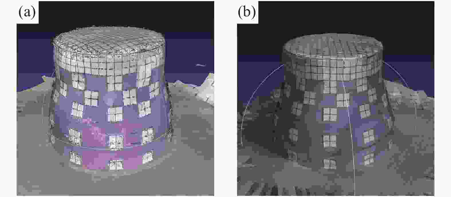
Figure 10.  Three-dimensional reconstruction of the lampshade

从图10中可以直观的看出，在上文所述覆盖率和精度的评估标准下，球形测量网络和椭球形测量网络均能够完整的还原待测物基本三维全貌，待测物表面粘贴的标志点也能清晰显示。但受限于当前三维重建算法不够精确，对于部分特征点未能完全匹配，导致待测物表面部分线条不连贯，而且实验室测量装置条件有限，无法完全满足视觉传感器采集图像信息的要求，致使重建待测物三维形貌不完善，但实验结果仍能够表明，椭球形测量网络相较于球形网络在所需相机数目和测量效率上仍具有较大优势。在后续的研究工作中，将会以三维重建为重点，进一步优化重建算法，考虑更全面的约束条件，使测量装置达到采集要求，为立体视觉测量组网技术提供研究支撑。

针对机器视觉三维测量，提出一种多视点立体视觉测量组网方法，在保证覆盖率和高精度的情况下，使测量所需相机数目达到最小化。相对于传统的SFM三维测量方法，所提出方法能够实现全覆盖测量，精度较高且成本较低。在验证实验中，与球形网络进行对比，该方法优化下的椭球形测量网络在相机数目、覆盖率和测量精度上均明显优于已有方法。最后据优化结果进行了三维重建，与实物图相比，基本还原了待测物全貌。在所提出多视点立体视觉测量组网方法的基础上，后续应进一步考虑待测物模型获取方法与约束条件，以实现组网方法的泛化性。