


-
视频监控系统越来越多地出现在各种公共场景和私人场所中,以监控人类活动并防止犯罪发生。毫无疑问,这需要有人观看监控视频,并在发生与正常情况不同的事情时进行判断并发出警报。然而,这些异常事件并不经常发生,因此大多数时候监控这些视频的人不会看到任何异常行为。这些不寻常的事件可以被认为是异常,可以将其定义为不符合正常情况的模式,发现这些不符合正常模式的任务称为异常检测。基于此,研究人员一直在尝试设计一种强大的异常检测算法,以自动监控和检测监控视频中的异常事件。
异常检测是一项具有挑战性的任务[1]:首先,异常事件的定义往往取决于当时的环境,很难准确地区分正常事件和异常事件。其次,构成异常的不同可能性是无限的。第三,异常数据点,尤其是真实世界的数据,往往与可能被定义为正常的数据点非常接近。这些原因导致异常检测任务十分困难,是过去几年研究人员在提出新解决方案时一直在考虑的问题。
近十年前,大多数研究人员都专注于基于轨迹的异常检测[2-3]。主要思想是:如果感兴趣的对象没有符合学习到的正常轨迹模式,视频将被标记为异常。然而,这种方法的一个主要缺点是遮挡,因为该方法严重依赖于持续检测跟踪感兴趣的对象。由于这些缺点,研究者们开始采用底层特征进行特征提取。这些基于低级特征的方法依赖于外观、运动和纹理特征的使用[4-6]。大量的方法已经使用了各种底层运动特征表示来表示视频,如社会力模型、光流直方图等,但是这些仅基于运动的特征是不够充分的。动态纹理、描述空间和运动的光流特征、光流空间局部直方图和基于均匀局部梯度模式的光流等特征被提出[6-7]。
尽管这些传统方法在基准数据集上取得了成功,但泛化能力较差,在其他场景中使用时它们仍然无效。此外,它们无法适应以前从未见过的异常。由于这些原因,研究人员探索使用深度神经网络来完成异常检测任务。这些神经网络能够自动学习有用的判别特征,从而消除了创建手工特征的麻烦,这也使其在用于不同场景时更具适应性。深度学习被证明对各种计算机视觉任务有效[8-9],例如图像中的特征提取、图像分类、对象检测、视频分析和许多其他任务。深度学习技术主要侧重于创建新网络结构或设计适合特定问题的组件。现有的基于深度学习的视频异常检测方法可以分为四类:(1)基于重构的方法[10-11]:这类方法假设是正常样本的重构误差会更低,因为它们更接近训练数据,而对于不正常的样本,假设或预期重建误差会更高。这类方法往往基于自编码,它能够将输入编码为更紧凑的表示的同时保留重要的判别特征,并且还能够将该特定编码解码回其原始形式。(2)基于预测未来帧的方法[12-13]:这类方法主要是通过对基于现有帧对未来帧进行预测,看其是否符合现有帧的模式进行异常判断。这类方法基于生成对抗网络,它包含生成器和鉴别器两个网络,前者能够模拟原始数据分布,后者则给出输入是否来自生成器的概率。(3)基于分类的方法[14-15]:这类问题可以看成对一段视频片段进行直接分类,给出其正常或是异常类别。由于正负例训练样本不在一个数量级,这类方法集中于利用卷积神经网络创建紧凑、高效且鲁棒的特征。(4)基于异常得分的方法[16-23]:将问题定义为回归问题,其中目标是提供异常分数,然后将其用作确定视频片段或帧是否异常的手段。
与这些方法不同的是,文中基于深度自编码高斯混合模型(deep autoencoding Gaussian mixture model,DAGMM),提出一种新的异常检测方法。DAGMM包含一个压缩网络和一个估计网络:压缩网络通过深度自动编码器对输入视频片段进行降维,根据低维特征和重构误差特征输入到估计网络中;而估计网络则通过高斯混合模型预测能量概率,然后通过能量密度概率判断异常。通过同时最小化来自压缩网络的重建误差和来自估计网络的样本能量,可以联合训练一个降维结构,直接帮助目标密度估计任务。与之前方法不同的是,文中方法能够同时对事件表示(压缩网络)和异常检测模型(估计网络)进行联合优化,泛化能力强。在几个公共基准数据集上的实验表明,DAGMM的性能检测效果达到现有技术发展水平。
-
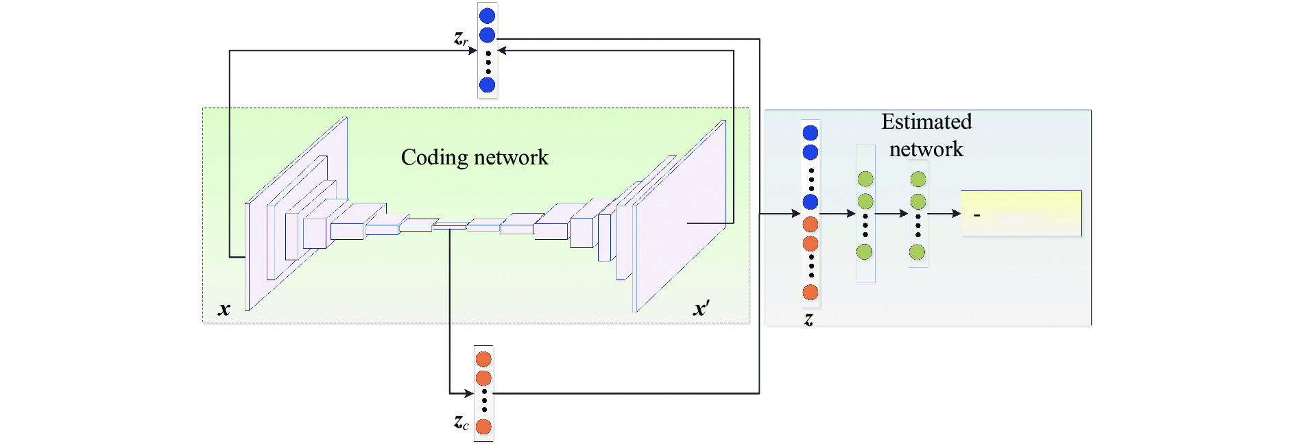
图1为DAGMM的整体网络结构,分两个子结构,左边部分为压缩网络,是一个深度全卷积自编码网络,通过这个自编码可以得到输入视频块
${\boldsymbol{x}}$ 的低维表示${{\boldsymbol{z}}_r}$ ,同时得到输入${\boldsymbol{x}}$ 与重构的${\boldsymbol{x}}'$ 之间的重构误差${{\boldsymbol{z}}_c}$ ,然后进行拼接操作形成${\boldsymbol{z}}$ ;右边为估计网络,也是一个多层的全连接前馈神经网络,输入为${\boldsymbol{z}}$ ,经过多层全连接得到一个概率分布,这个概率分布的长度即为混合高斯分布中高斯成分的个数。那么可以通过这个输出概率判断输入是否为异常。
图 1 基于深度自编码-高斯混合模型的异常检测方法流程
Figure 1. Flow chart of abnormal event detection method based on DAGMM
-
如图1所示,压缩网络提供的低维表示包含两个特征来源:(1)深度自编码器学习到的低维表示;(2)由重构误差导出的特征。给定一个样本
${\boldsymbol{x}}$ ,压缩网络计算其低维表示${\boldsymbol{z}}$ 如下:$$ {{\boldsymbol{z}}_c}{\text{ = }}{f_{{w_{\text{1}}}}}\left( {\boldsymbol{x}} \right) $$ (1) $$ {\boldsymbol{x}}'{\text{ = }}{g_{{w_2}}}\left( {{{\boldsymbol{z}}_c}} \right) $$ (2) $$ {{\boldsymbol{z}}_r}{\text{ = }}h\left( {{\boldsymbol{x}},{\boldsymbol{x}}'} \right) $$ (3) $$ {\boldsymbol{z}}{\text{ = }}\left[ {{{\boldsymbol{z}}_c},{{\boldsymbol{z}}_r}} \right] $$ (4) 式中:
${\boldsymbol{x}}$ 和${\boldsymbol{x}}'$ 分别为自编码器的输入和重构的输入(即自编码器的输出);${{\boldsymbol{z}}_r}$ 为${\boldsymbol{x}}$ 的隐层表示;${w_1}$ 和${w_2}$ 为自编码网络中编码器和解码器的参数;$ h( \cdot , \cdot ) $ 表示计算重构误差的函数。然后,获得的特征${\boldsymbol{z}}$ 被传入估计网络中。 -
给定输入样本的低维表示
${\boldsymbol{z}}$ ,估计网络在高斯混合模型(Gaussian mixture model,GMM)的框架下进行密度估计。与传统GMM不同的是,估计网络在训练阶段无需采用期望最大化(expectation-maximization, EM)算法中的交替迭代的方法,通过未知混合分量分布$ \phi $ 、混合均值$\; \mu $ 和混合协方差$ \Sigma $ 即可直接估计GMM 的参数并评估样本的似然。为了实现这一点,估计网络通过利用多层神经网络来预测每个样本的混合成分。给定特征${\boldsymbol{z}}$ 和混合成分的个数特征$ K $ ($ K $ 的大小将在2.3节中进行讨论),则样本属于高斯混合分布中各个分布的概率为:$$ {\boldsymbol{p}}{\text{ = }}MLN\left( {{\boldsymbol{z}};{\theta _m}} \right) $$ (5) $$ {\overset{\frown} \gamma} {\text{ = softmax}}\left( {\boldsymbol{p}} \right) $$ (6) 式中:
${\overset{\frown} \gamma}$ 表示预测结果,是个$ K $ 维的向量;${\boldsymbol{p}}$ 为多层感知器的输出。给定$ N $ 个样本和预测结果,那么可以估计出GMM的参数如下:$$ {{\overset{\frown} \phi} _k}{\text{ = }}\sum\limits_{i = 1}^N {\frac{{{{\overset{\frown} \gamma}_{ik}}}}{N}} $$ (7) $$ {{\overset{\frown} \mu} _k}{\text{ = }}\frac{{\displaystyle\sum\limits_{i = 1}^N {{{{\overset{\frown} \gamma} }_{ik}}{{\boldsymbol{z}}_i}} }}{{\displaystyle\sum\limits_{i = 1}^N {{{{\overset{\frown} \gamma} }_{ik}}} }} $$ (8) $$ {{\overset{\frown} \Sigma} _k}{\text{ = }}\frac{{\displaystyle\sum\limits_{i = 1}^N {{{{\overset{\frown} \gamma} }_{ik}}\left( {{{\boldsymbol{z}}_i} - {{{\overset{\frown} \mu} }_k}} \right){{\left( {{{\boldsymbol{z}}_i} - {{{\overset{\frown} \mu} }_k}} \right)}^{\rm{T}}}} }}{{\displaystyle\sum\limits_{i = 1}^N {{{{\overset{\frown} \gamma} }_{ik}}} }} $$ (9) 式中:
$ {{\overset{\frown} \gamma} _i} $ 为隐层表示${{\boldsymbol{z}}_i}$ 属于第$ i $ 个分量的概率;${{\overset{\frown} \phi } _k},{{\overset{\frown} \mu} _k},{{\overset{\frown} \Sigma} _k}$ 分别表示GMM中第$k$ 个成分的混合概率、均值和方差。那么,样本的概率分布可以表示为:$$ E({\boldsymbol{z}}){\text{ = }} - {\text{log}}\left( {\sum\limits_{k = 1}^k {{{{\overset{\frown} \phi } }_k}\frac{{\exp \left( { - \dfrac{1}{2}{{\left( {{{\boldsymbol{z}}_i} - {{{\overset{\frown} \mu} }_k}} \right)}^{\rm{T}}}\Sigma _k^{ - 1}\left( {{{\boldsymbol{z}}_i} - {{{\overset{\frown} \mu} }_k}} \right)} \right)}}{{\sqrt {\left| {2\pi {{{\overset{\frown} \Sigma} }_k}} \right|} }}} } \right) $$ (10) 其中,
$ \left| \cdot \right| $ 表示矩阵的行列式。 -
基于以上压缩网络和估计网络的基本原理,DAGMM的的目标函数可以表示为:
$$ J\left( {{W_1},{W_2},{\theta _m}} \right){\text{ = }}\frac{1}{N}\sum\limits_{i = 1}^N {L\left( {{{\boldsymbol{x}}_i},{{{\boldsymbol{x}}'}_i}} \right)} + \frac{{{\lambda _1}}}{N}\sum\limits_{i = 1}^N {E\left( {{{\boldsymbol{z}} _i}} \right)} + {\lambda _2}P\left( {{\overset{\frown} \Sigma} } \right) $$ (11) 式中:
$ N $ 为训练样本个数;$ {\lambda _1} $ 和$ {\lambda _2} $ 为用于平衡三项的参数。目标函数共包含三项,第一项中$L\left( {{{\boldsymbol{x}}_i},{{{\boldsymbol{x}}'}_i}} \right)$ 为压缩网络中深度自编码器造成的重构误差的损失函数。如果压缩网络能够使重构误差较低,那么低维表示可以更好地保留输入样本的关键信息;第二项$E\left( {{{\boldsymbol{z}} _i}} \right)$ 是可以观察到输入样本的概率。通过最小化样本概率,可以通过寻找压缩和估计网络的最佳组合,以最大化观察输入样本的可能性;第三项是惩罚项,防止矩阵不可逆。 -
对于给定的测试样本
$ y $ ,如果其为正常样本,那么一定能够和某个(某几个)高斯分量相关联,因此其隐层表示属于某个高斯分量的条件概率一定会相对比较大。反之,异常样本无法与任何一个高斯分量相关联,那么其属于所有高斯分量的条件概率都很小。在预测阶段,首先根据公式(1)、(3)、(4)获得其隐层表示
${{\boldsymbol{z}}_y}$ ,然后通过公式(10)计算隐层表示${{\boldsymbol{z}}_y}$ 的能量,并设定门限值$ \xi $ 判断其是否为异常:$$ E({{\boldsymbol{z}}_y}) > \xi $$ (11) -
为了验证文中提出的方法,在两个公开可用的视频异常数据集上评估提出的方法,即UCSD PED1行人数据集[4]和ShanghaiTech[18]校园数据集。这两个数据集都有自己的挑战和独特的特征,例如异常类型、视频质量、背景位置等,两个数据集的简要介绍如表1所示。因此,需要对两个数据集分别训练模型并进行测试。
UCSD行人异常检测数据集由Mahadevan等人创建的,目的是评估他们的异常检测方法。该数据集包含由安装在高处的固定相机以10帧/s的速度拍摄的俯瞰人行道的视频。在这个数据集中,异常事件包括人行道上的非行人和异常的行人运动,具体来说,一些异常示例包括骑自行车的人、溜冰者、猫等。该数据集有两个子集,其中每个子集对应于特定场景。文中仅采用第一个场景即UCSD PED2进行实验,包含16个训练片段和14个测试片段,共4560帧,分辨率为320×240。
ShanghaiTech数据集的提出是由于现有基准数据集缺乏场景多样性。与之前的数据集相比,ShanghaiTech数据集的视频数量更多,总共有330个训练视频和107个测试视频,包括13个不同的场景和大量不同的异常类型。该数据集中视频的分辨率为856×480。此外,异常事件包括人行道上自行车、追逐和争吵等突然运动引起的异常。
帧级评价指标被用于评估检测方法的性能。对于帧级评价指标来说,如果一个帧的至少一个像素被标记为异常,则该帧被认为是异常的。为了使用帧级标准进行评估,时间标签用于确定度量标准的真阳性和假阳性,并通过公式(12)和公式(13)来计算方法的检测率(true positive rate,TPR)和虚警率(false positive rate,FPR):
$$ TPR = \frac{{TP}}{{TP + FN}}\; $$ (12) $$ FPR = \frac{{FP}}{{FP + TN}}\; $$ (13) 对于这两个标准,计算接收者操作特征曲线 (ROC)的曲线下面积 (AUC) 以衡量模型的最终性能。给定具有不同阈值的分类模型,接收者操作特征曲线 (ROC) 说明了模型的性能。
-
对于两个数据集,每帧都被调整为大小420×280,且转换为灰度图。网络的输入为28×28×3长方体,意味着420×280×3的连续3帧视频可以划分为15×10的长方体。压缩网络中编码器的结构类似于参考文献[19]中的 Model C。CNN的结构采用常见的C64×(3×3)−C128×(3×3)−C256×(3×3)−C64×(4×4)的结构,即首先为64个大小3×3卷积核的卷积层,接下来采用128个大小3×3卷积核的卷积层,然后采用256个大小3×3卷积核的卷积层和256个大小4×4卷积核的卷积层,可以获得256维的向量
${{\boldsymbol{z}}_c}$ 。解码器的网络结构与编码器相反,而重构向量${{\boldsymbol{z}}_{\text{r}}}$ 为2352维,因此预测网络的输入为2608维,其中全连接层网络节点数目分别设置为500和50,输出层为softmax层,所有的激励函数均设置为tanh。公式(11)中$ {\lambda _1} $ 和$ {\lambda _2} $ 分别设置为0.1和0.01,公式(5)中$ K $ 设置为16。整个模型参数优化选取的是Adam优化器,初始学习率为0.0001,迭代次数为1000。动量(momentum)参数为$ {\rho _1}{\text{ = }}0.9,{\rho _2} = 0.999 $ ,批尺寸为128。实验硬件平台为NVIDIA GTX1070TI,显存8 GB,软件环境为Tensorflow 1.15和Python 3.6。 -
为了验证文中提出方法的优势,将所提出的方法同十余种方法进行了对比。这些方法包含采用手工特征的方法,如MPPCA[3]、动态纹理(MDT)[4]、MT-FRCN[5]等;也包括采用深度学习特征的方法,如包括2D卷积自动编码器方法(Conv2D-AE)[10]、3D 卷积自动编码器方法(Conv3D-AE)[10]、基于卷积长短时记忆网络的自动编码器方法(ConvLSTM-AE)[20]、堆叠循环神经网络 (StackRNN)[21]和基于生成对抗网络的方法(GAN)[18]。
表2以帧级AUC的形式给出了两个数据集的检测结果。通过表1可以看出,文中提出的方法优于其他对比方法。与基于手工特征的方法相比,所提出方法的结果在UCSD Ped2数据集上的准确率至少提高了3.5%帧级AUC(95.7% vs 92.2%)。值得注意的是,由于ShanghaiTech是近几年提出的新数据集,帧数较多,对于计算需求也比较大,目前为止没有基于手工特征的方法在该数据集上进行验证。与同深度学习的方法相比,文中提出的方法在两个数据集上取得了最佳的检测结果。具体来说,提出的方法在 UCSD Ped2 数据集和ShanghaiTech数据集上分别比Baseline[18]方法好0.3%和0.1%帧级AUC。但是,提出的方法在ShanghaiTech数据集上取得72.9%帧级AUC,相对于在UCSD Ped2数据集取得的95.7%帧级AUC来说要低很多,这主要是因为ShanghaiTech数据集相对于UCSD Ped2数据集更为复杂,包含多场景、多帧数、以及此前其他数据集中未出现的异常事件。
表 2 与现有技术发展水平检测方法结果对比(以AUC%的形式)
Table 2. Comparison with the state of the art methods in terms of AUC%
表 1 基准数据集概述
Table 1. Overview of benchmark datasets
Attributes UCSD Ped2 ShanghaiTech Frames 4560 317398 Scene Single Multi Labels Spatial & Temporal Spatial & Temporal Resolution 360×240 856×480 Anomalies Biker, cart, etc Chasing, brawling
sudden motion, etc为了评估公式(5)中预先定义了高斯混合分量个数
$ K $ 在检测视频异常事件方面的性能,通过改变高斯混合分量个数$ K $ 并在UCSD Ped2数据集上进行实验,实验结果以帧级AUC的形式给出。表3为在UCSD Ped2数据集上的检测结果。可以看出,当K<16时,检测结果随着$ K $ 值增大而提升,这主要是因为较小的$ K $ 值导致原本区别很大的样本被聚集在同一个高斯混合分量下,损失了较多的局部细节信息;而当$K > 16$ 时,检测性能不再随着$ K $ 值增大而变化。但是,根据公式(7)~(9),采用较大的$ K $ 值会导致更大的计算量。表 3 高斯混合分量个数K对于UCSD Ped2数据集实验结果(帧级 AUC%)的影响
Table 3. Influence of the number of Gaussian mixture components number K on the experimental results of the UCSD Ped2 data set (frame-level AUC%)
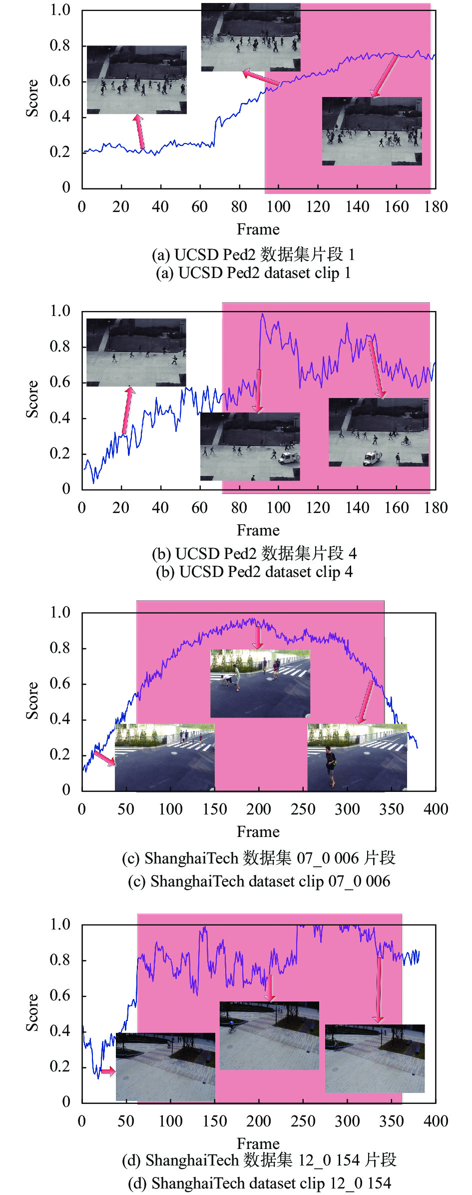
$ K $ AUC% 2 92.3% 4 94.5% 8 951% 16 95.7% 32 95.6% 64 95.7% 图2(a)~(d)分别展示了文中提出的方法在UCSD Ped2数据集和ShanghaiTech数据集中的一些视频片段上估计的帧级异常分数。其中,横坐标为视频帧数,纵坐标异常分数已经归一化到1,红色区域表示真实注释的异常帧。通过图2可以看出,异常得分较大的区域和真实标注的异常帧能够基本吻合上,一些异常事件如人行道上出现自行车、小车,打架推搡基本能够检测出。此外,图2还提供了一些具有正常或异常事件的关键帧。当异常事件突发,如图2(b)场景中出现小车时,异常得分突然增加;相反,如果导致异常的对象在摄像头视野中消失,如图2(c)所示,则异常得分会降低。

图 2 部分检测结果示例
Figure 2. Examples of the detection results
-
文中提出了一种DAGMM网络,结合了深度自编码和高斯混合模型,用于监控视频中的异常检测。DAGMM由两个主要部分组成:压缩网络和估计网络,其中压缩网络将样本投影到低维空间,保留异常检测的关键信息,估计网络在框架下评估低维空间中的样本能量高斯混合建模。DAGMM能够实现端对端训练,估计网络预测样本混合隶属度,从而无需交替程序即可估计GMM中的参数,估计网络引入的正则化有助于压缩网络摆脱吸引力较小的局部最优,并通过端到端训练实现低重构误差。在两个数据集上的实验证明了文中提出的方法与最先进的方法相比具有竞争力。
A video anomaly detection method based on deep autoencoding Gaussian mixture model
-
摘要: 由于异常定义的模糊性和真实数据的复杂性,视频异常检测是智能视频监控中最具挑战性的问题之一。基于自动编码器(AE)的帧重建(当前或未来帧)是一种流行的视频异常检测方法。使用在正常数据上训练的模型,异常场景的重建误差通常比正常场景的重建误差大得多。但是,这类方法忽略了正常数据本身的内部结构,效率较低。基于此,提出了一种深度自动编码高斯混合模型(DAGMM)。首先利用深度自动编码器获得输入视频片段的生成低维表示和重构误差,并将其进一步输入高斯混合模型(GMM)。而估计网络则通过高斯混合模型预测能量概率,然后通过能量密度概率判断异常。DAGMM以端到端的方式同时联合优化深度自动编码器和GMM的参数,能够平衡自动编码重建、低维表示的密度估计和正则化,泛化能力强。在两个公共基准数据集上的实验结果表明,DAGMM达到了现有最高技术发展水平,在UCSD Ped2和ShanghaiTech两个数据集上分别取得了95.7%和72.9%的帧级AUC。Abstract: Due to the vagueness of anomaly definition and the complexity of real data, video anomaly detection is one of the most challenging problems in intelligent video surveillance. Frame reconstruction (current or future frame) based on autoencoder (AE) is a popular video anomaly detection method. Using a model trained on normal data, the reconstruction error of abnormal scenes is usually much larger than that of normal scenes. However, these methods ignore the internal structure of the normal data and are memory-consuming. Based on this, a deep auto-encoding Gaussian mixture model (DAGMM) was proposed. Firstly, the deep autoencoder was used to obtain the low-dimensional representation of the input video segment and the reconstruction error, and then further input into a Gaussian mixture model (GMM). The energy probability was predicted through the Gaussian mixture model, and then the anomaly was judged through the energy density probability. The proposed DAGMM can simultaneously optimizes the parameters of the deep autoencoder and GMM in an end-to-end manner, and balance auto-encoding reconstruction, density estimation and regularization of low-dimensional representation, and has strong generalization ability. Experimental results on two public benchmark datasets show that DAGMM has reached the highest level of technological development, achieving 95.7% and 72.9% frame-level AUC on the UCSD Ped2 and ShanghaiTech dataset, respectively.
-
Key words:
- video surveillance /
- anomalous event /
- auto-encoding network /
- Gaussian mixture model /
- deep learning
-
图 1 基于深度自编码-高斯混合模型的异常检测方法流程
Figure 1. Flow chart of abnormal event detection method based on DAGMM
表 2 与现有技术发展水平检测方法结果对比(以AUC%的形式)
Table 2. Comparison with the state of the art methods in terms of AUC%
 下载: 导出CSV
表 1 基准数据集概述
Table 1. Overview of benchmark datasets
Attributes UCSD Ped2 ShanghaiTech Frames 4560 317398 Scene Single Multi Labels Spatial & Temporal Spatial & Temporal Resolution 360×240 856×480 Anomalies Biker, cart, etc Chasing, brawling
sudden motion, etc
下载: 导出CSV
表 3 高斯混合分量个数K对于UCSD Ped2数据集实验结果(帧级 AUC%)的影响
Table 3. Influence of the number of Gaussian mixture components number K on the experimental results of the UCSD Ped2 data set (frame-level AUC%)
$ K $ AUC% 2 92.3% 4 94.5% 8 951% 16 95.7% 32 95.6% 64 95.7%
下载: 导出CSV
-
[1] Sabokrou M, Fayyaz M, Fathy M, et al. Deep-anomaly: Fully convolutional neural network for fast anomaly detection in crowded scenes [J]. Computer Vision and Image Understanding, 2018, 172: 88-97. doi: 10.1016/j.cviu.2018.02.006 [2] Li C, Han Z, Ye Q, et al. Visual abnormal behavior detection based on trajectory sparse reconstruction analysis [J]. Neurocomputing, 2013, 119(7): 94-100. [3] Jiang F, Yuan J, Tsaftaris S A, et al. Anomalous video event detection using spatiotemporal context [J]. Computer Vision and Image Understanding, 2011, 115(3): 323-333. doi: 10.1016/j.cviu.2010.10.008 [4] Li W, Mahadevan V, Vasconcelos N. Anomaly detection and localization in crowded scene [J]. IEEE Transactions on Pattern Analysis and Machine Intelligence, 2014, 36(1): 18-32. [5] Reddy V, Sanderson C, Lovell B. Improved anomaly detection in crowded scenes via cell-based analysis of foreground speed, size and texture [C]//IEEE Computer Society Conference on Computer Vision and Pattern Recognition Workshops (CVPRW), 2011: 55-61. [6] Wang S, Zhu E, Yin J, et al. Video anomaly detection and localization by local motion based joint video representation and OCELM [J]. Neurocomputing, 2018, 277: 161-175. doi: 10.1016/j.neucom.2016.08.156 [7] Kaur P, Gangadharappa M, Gautam S. An overview of anomaly detection in video surveillance [C]//International Conference on Advances in Computing, Communication Control and Networking (ICACCCN), 2018. [8] Schmidhuber J. Deep learning in neural networks: An overview [J]. Neural Networks, 2015, 61: 326-366. [9] Lecun Y, Bengio Y, Hinton G. Deep learning [J]. Nature, 2015, 521: 436-444. doi: 10.1038/nature14539 [10] Hasan M, Choi J, Neumanny J, et al. Learning temporal regularity in video sequences [C]//Proceedings of IEEE Conference on Computer Vision and Pattern Recognition, 2016: 770-778. [11] Gong D, Liu L, Le V, et al. Memorizing normality to detect anomaly: Memory-augmented deep autoencoder for unsupervised anomaly detection [C]//IEEE/CVF Conference on Computer Vision and Pattern Recognition, 2019: 1-8. [12] Ravanbakhsh M, Sangineto E, Nabi M, et al. Abnormal event detection in videos using generative adversarial nets [C]//Proceedings of the IEEE International Conference on Image Processing (ICIP) 2017: 1-5. [13] Ravanbakhsh M, Sangineto E, Nabi M, et al. Training adversarial discriminators for cross-channel abnormal event detection in crowds [C]//Winter Conference on Applications of Computer Vision, 2019: 1896-1904. [14] Narasimhan MG, S SK. Dynamic video anomaly detection and localization using sparse denoising autoencoders [J]. Multimedia Tools Appl, 2018, 77(11): 1317313195. [15] Sabzalian B, Marvi H, Ahmadyfard A. Deep and sparse features for anomaly detection and localization in video [C]//4th International Conference on Pattern Recognition and Image Analysis (IPRIA), 2019: 173-178 [16] Lin S, Yang H, Tang X, et al. Social MIL: Interaction-aware for crowd anomaly detection [C]//16th IEEE International Conference on Advanced Video and Signal Based Surveillance (AVSS), 2019: 1-8. [17] Fan Y, Wen G, Li D, et al. Video anomaly detection and localization via gaussianmixture fully convolutional variational autoencoder [J]. Computer Vision and Image Understanding, 2020, 195: 102920. doi: 10.1016/j.cviu.2020.102920 [18] Liu W, Luo W, Lian D, et al. Future frame prediction for anomaly detection-a new baseline [C]//IEEE/CVF Conference on Computer Vision and Pattern Recognition, 2018: 6536-6545. [19] Springenberg J, Dosovitskiy A, Brox T, et al. Striving for simplicity: The all convolutional net [C]//International Conference on Learning Representations, 2015. [20] Luo W, Liu W, Gao S. Remembering history with convolutional lstm for anomaly detection [C]//IEEE International Conference on Multimedia and Expo (ICME), 2017: 439-444. [21] Luo W, Liu W, Gao S. A revisit of sparse coding based anomaly detection in stacked rnn framework [C]//IEEE International Conference on Computer Vision, 2017: 341-349. [22] 王栋, 张晓俊, 戴丽华. 基于深度高斯过程回归的视频异常事件检测方法[J]. 电子测量与仪器学报, 2021, 35(3): 158-164 Wang Dong, Zhang Xiaojun, Dai Lihua. Video anomaly detection and localization via deep Gaussian process regression [J]. Chinsese Journal of Scientific Instrument, 2021, 35(3): 158-164. (in Chinese) [23] 佘博, 田福庆, 梁伟阁. 基于深度卷积变分自编码网络的故障诊断方法[J]. 电子测量与仪器学报, 2018, 39(10): 27-35 Yu Bo, Tian Fuqing, Liang Weige. Fault diagnosis based on a deep convolution variational autoencoder network [J]. Journal of Electronic Measurenment and Instrument, 2018, 39(10): 27-35. (in Chinese) -

 点击查看大图
计量
- 文章访问数: 336
- HTML全文浏览量: 78
- PDF下载量: 29
- 被引次数: 0


