


-
目标检测是进行场景内容理解等高级视觉任务的前提,已广泛应用于智能视频监控、基于内容的图像检索、视觉导航等任务中。传统的目标检测主要使用人工设计的特征(如HAAR[1]、HOG[2]、SIFT[3]、SURF[4]等),在滑动窗口下使用分类器进行判别,其代表方法有Adaboost-SVM[5]和形变部件模型(DPM)[6-8]。上述方法开创了实用化的目标检测之先河,在便携式设备和机器人等领域有着广泛应用。但由于人工设计特征的性能所限,传统方法的准确率始终不高,且通常对新的图像缺乏足够的泛化能力。
相比传统目标检测方法,基于卷积神经网络(CNN)的目标检测方法在准确率方面具有显著优势。CNN通过大量参数拟合各类不同的情形,使用多层架构逐步抽象目标信息,极大地提升了目标检测的泛化能力。然而当前基于CNN的目标检测相关研究集中于RGB图像目标检测以及通用图像目标检测,而对红外目标检测的深度学习方法研究相对较少。两个重要的原因在于:(1)公开的红外图像数据集数量远远少于RGB图像数据集数量;(2)红外数据集的规模通常较小,标注数据不充分。上述问题导致深度学习方法的训练样本不足,算法测试困难,严重制约了基于深度学习的红外目标检测技术的发展。针对上述问题,文中结合迁移学习与半监督学习,旨在使用少量的已标注红外图像训练精度较高的红外目标检测网络。
迁移学习(Transfer learning)指的是将一个任务中的预训练模型(经过少许训练)重新用在另一个任务当中。深度学习中的这种迁移被称作归纳迁移,就是通过使用一个适用于不同但是相关的任务的模型,以一种有利的方式缩小可能模型的搜索范围[9]。在目标检测任务中,参考文献[10]将ImageNet[11]中训练的分类网络的中级特征迁移到目标检测网络中,成功提高了目标检测精度;参考文献[12]在STL-10中通过无监督训练学习图像的局部特征,并迁移到无人机目标识别网络中。鉴于上述成功案例可预计,在红外目标检测中使用大型RGB数据集的预训练模型有望显著降低训练所需样本规模以及训练量,提高模型的收敛速度。
半监督学习(Semi-supervised Learning, SSL)是监督学习与无监督学习相结合的一种学习方法,其同时使用大量的未标记数据和部分标记数据进行模式识别工作,已经成功用于RGB图像的两阶段目标检测网络[13]和SAR目标检测网络[14]的训练中。参考文献[15]为两阶段目标检测网络的半监督训练引入噪声扰动下的自监督损失,进一步提高了目标检测的准确率。相比于全监督学习(Supervised learning),半监督学习利用了额外的无标注数据所提供的样本的分布信息,从而使模型拟合更为真实的数据分布,提高模型的泛化能力。在红外目标检测网络的训练中,半监督学习能够充分利用无标注的红外图像特征分布,解决目标检测网络由于红外图像数据集规模较小、标注不充分所引起的过拟合问题,提高其在测试当中的检测精度。
综合考虑红外数据集规模小,标记样本少的特点,文中提出了一种红外目标检测网络的半监督迁移学习方法,主要用于提高目标检测网络在小样本红外数据集上的训练效率和泛化能力,提高深度学习方法在训练样本较少的红外目标检测场景当中的适应性。实验结果表明,该方法所训练的目标检测网络测试精度显著高于仅使用监督学习训练的网络,验证了所提出方法的有效性。
-
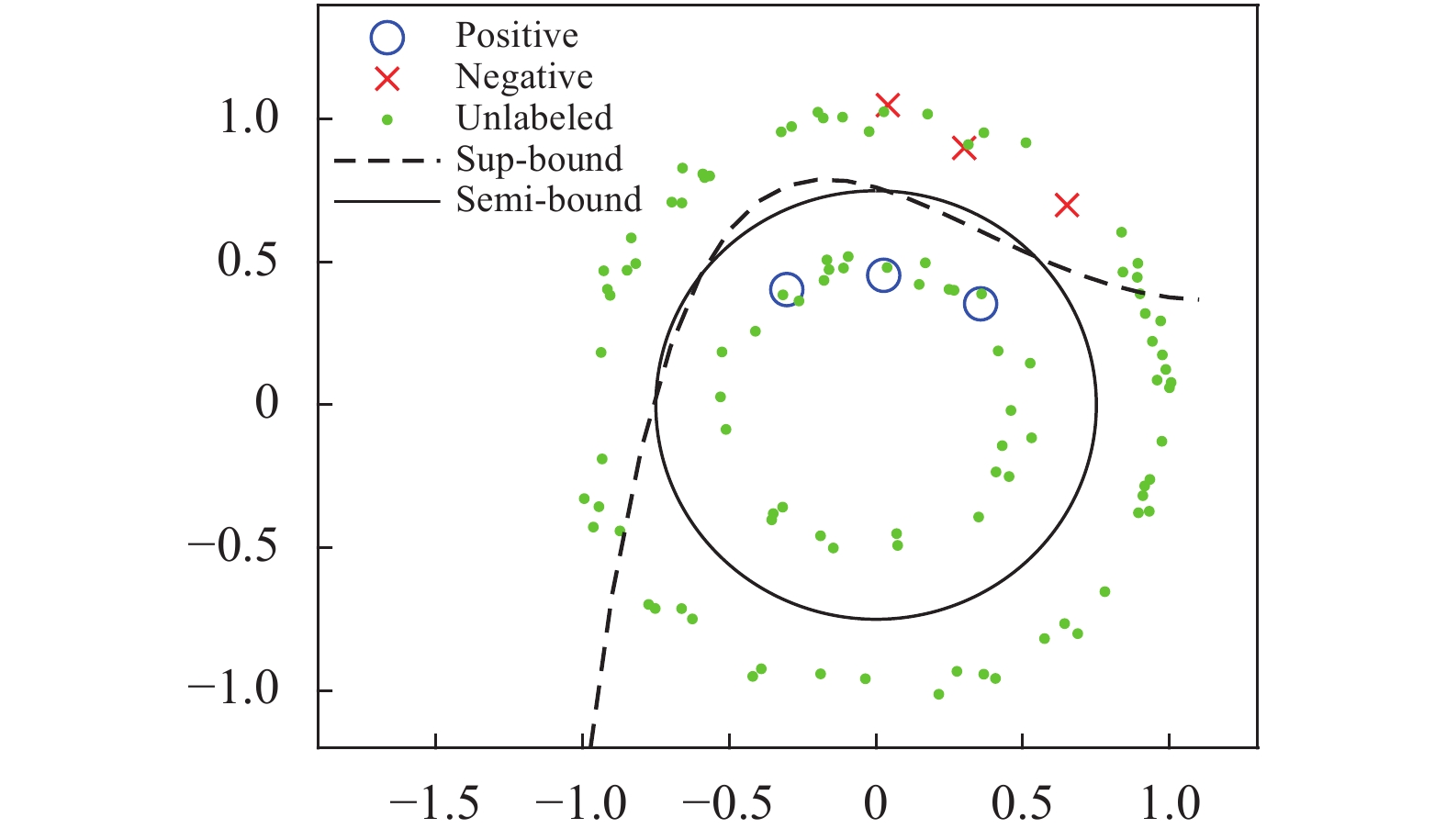
当标注样本足够多时足以表示任务数据的真实分布,此时通过全监督学习就足以训练较为理想的模型。而当标注样本不足时,这些样本可能无法表示任务数据的真实分布,此时单纯采用全监督学习容易造成模型对训练样本集的过拟合,同时对任务数据的真实分布欠拟合,从而出现训练准确率高、测试准确率低的问题;另一方面,训练样本过少使得模型对样本噪声和标注误差十分敏感,进一步降低了模型的稳定性。相比于全监督学习,半监督学习利用了无标注样本所提供的分布信息,使模型得以学习更为真实的数据分布,提高了模型的稳定性和泛化能力。为了直观地阐明该现象,图1例举了一个包含少量标注样本和无标注样本的二维分类问题。其中蓝色圆圈为正样本(Positive),红色叉为负样本(Negative),绿色点为无标注样本,Sup-bound为全监督模型的分类边界,Semi-bound为半监督模型的分类边界。可以看到,由于标注样本的分布偏差,全监督模型出现了过拟合,导致其在标注样本外的区域泛化能力严重下降;相比于全监督模型,半监督模型能够利用相对丰富的无标注样本获得数据分布信息,得到泛化性更好的分类结果。
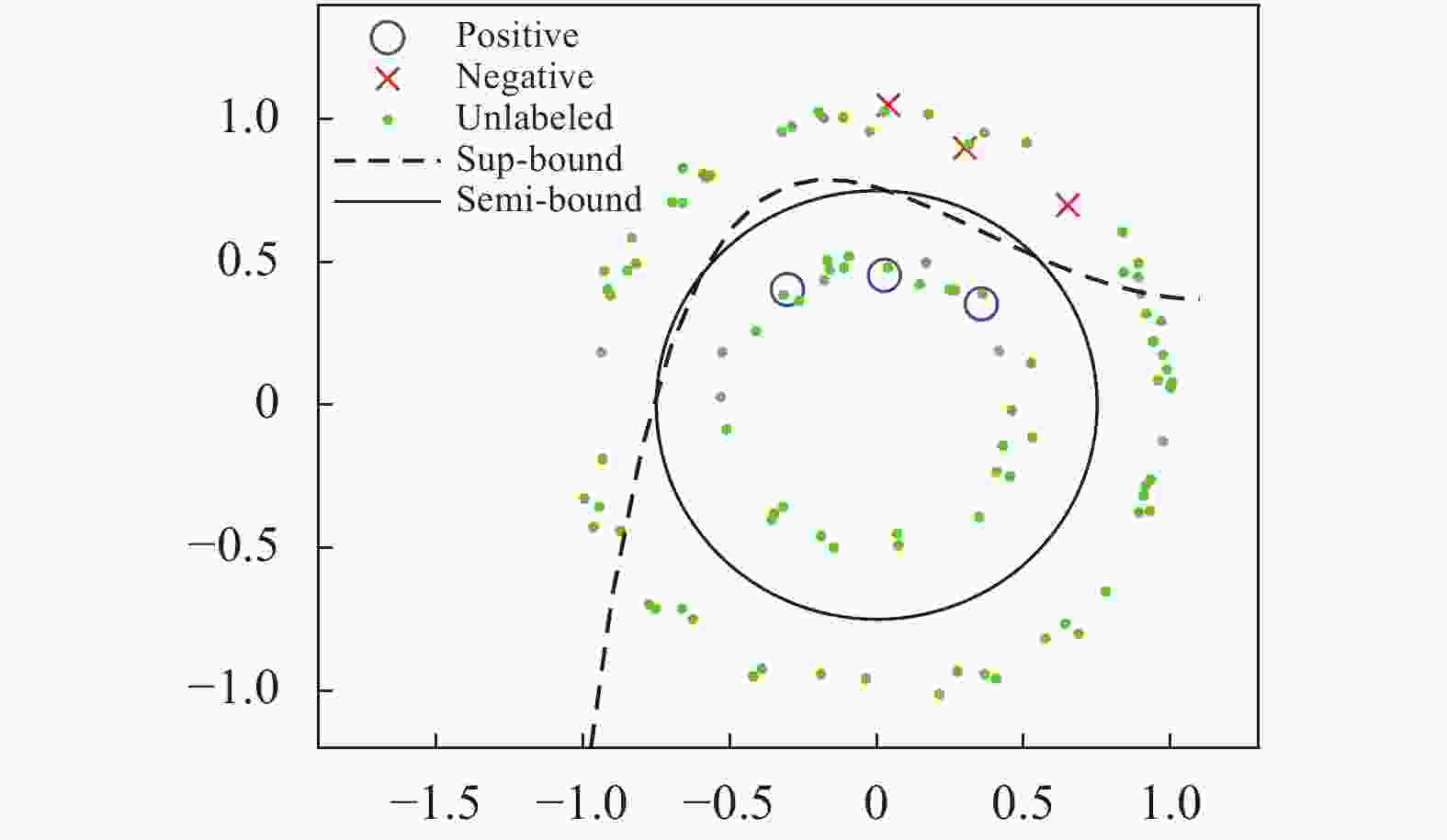
图 1 无标注样本对分类面的影响
Figure 1. Influence of unlabeled samples on decision boundary
-
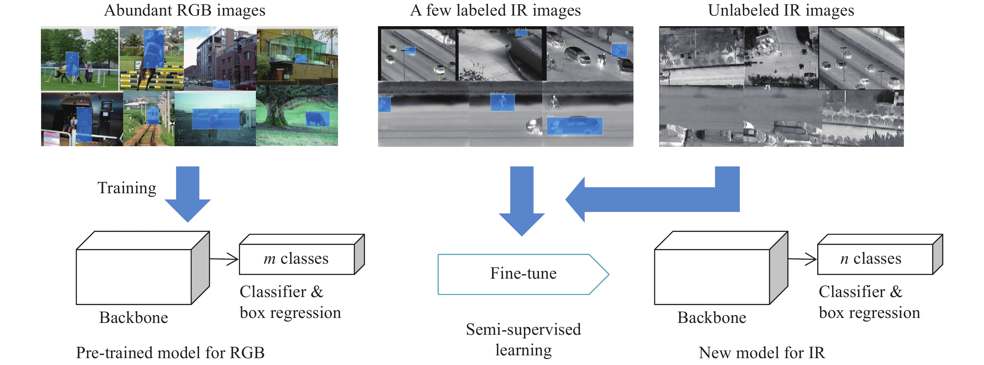
在图像领域,迁移学习常常用于将某个任务中学到的图像特征或高级语义信息初始化另一个任务的部分或全部模型,随后使用该任务的训练样本对模型进行微调。但在诸如红外目标检测等训练样本较少的任务中,由于训练样本自身的特征维度较高,少量样本无法反映该任务数据的真实分布,微调过程会同时存在对训练样本过拟合与对任务真实分布欠拟合的问题。根据第1节的讨论,该问题可以通过在少量的标注样本外引入无标注样本对目标检测网络进行半监督训练予以解决,从而提高目标检测网络的泛化能力。文中设计的目标检测网络训练流程如图2所示,首先使用大量的RGB图像对原始网络模型进程训练,获得预训练模型(Pre-trained model),随后使用少量的有标注红外图像和相对更多的无标注红外图像对模型进行半监督学习调优,最终得到红外目标检测模型(Model for infrared object detection)。该训练过程的重点问题包括:(1)如何为无标注数据设计损失函数以准确表示无标注样本与标注样本的相关性,以及无标注样本之间的相关性;(2)如何设计半监督训练策略,在充分利用无标注样本分布信息的前提下,降低无标注样本在网络训练初期常见的伪标注错误的干扰,提高网络训练的收敛速度。应当注意的是,若预训练网络的分类器的输出通道个数与红外目标的类别数不同时,需要对分类器输出通道个数进行调整,以匹配训练所用的标注信息。
图 2 红外目标检测网络的半监督迁移学习方法流程
Figure 2. Procedures of semi-supervised transfer learning of infrared object detection neural network
-
给定标注数据集
${{\cal{D}}_I} = \{ (I,\varsigma )\} $ ,传统的全监督损失${\cal{L}}^{{\sup }}$ 可表示为:$$ \begin{split} &{\cal{L}}^{{\sup }}({{\cal{D}}_I};{\theta ^{\rm{b}}},{\theta ^{{\rm{cls}}}},{\theta ^{{\rm{reg}}}}) =\\ & \frac{1}{{|{{\cal{D}}_I}|}}\sum\limits_{I \in {{\cal{D}}_I}} {\left[ {{L^{{\rm{cls}}}}(I,{\varsigma ^{{\rm{cls}}}};{\theta ^{\rm{b}}},{\theta ^{{\rm{cls}}}}) + {L^{{\rm{loc}}}}(I,{\varsigma ^{{\rm{loc}}}};{\theta ^{\rm{b}}},{\theta ^{{\rm{reg}}}})} \right]} \\ \end{split}$$ (1) 式中:
$|{{\cal{D}}_I}|$ 为集合${{\cal{D}}_I}$ 的元素个数;${L^{{\rm{cls}}}}$ 为分类误差的损失函数;Lloc为定位误差的损失函数;I为单幅有标注图像;$\varsigma $ 为对应标注信息;${\varsigma ^{{\rm{cls}}}}$ 为类别标注;${\varsigma ^{{\rm{loc}}}}$ 为位置标注;${\theta ^{{\rm{cls}}}}$ 为分类器参数,${\theta ^{{\rm{reg}}}}$ 为回归器参数;${\theta ^{\rm{b}}}$ 为目标检测网络除分类器和回归器之外的其余部分参数。与全监督损失函数对应的半监督目标检测损失
${\cal{L}}{ ^{{\rm{semi}}}}$ 可表示为:$$ \begin{split} &{\cal{L}}{^{{\rm{semi}}}}({{\cal{D}}_I},{{\cal{D}}_u};{\theta ^{\rm{b}}},{\theta ^{{\rm{cls}}}},{\theta ^{{\rm{reg}}}}) = \\ & {\cal{L}}{^{\sup }}({{\cal{D}}_I};{\theta ^{\rm{b}}},{\theta ^{{\rm{cls}}}},{\theta ^{{\rm{reg}}}}) + \alpha {\cal{L}}{^{{\rm{self}}}}({{\cal{D}}_I},{{\cal{D}}_u};{\theta ^{\rm{b}}},{\theta ^{{\rm{cls}}}},{\theta ^{{\rm{reg}}}}) \\ \end{split} $$ (2) 式中:
${{\cal{D}}_u}$ 为无标注图像的集合;${\cal{L}}{^{\sup }}$ 为满足公式(1)的有监督损失;${\cal{L}}{^{{\rm{self}}}}$ 为无监督损失;$\alpha $ 为无监督损失的加权因子。关于
${\cal{L}}{^{{\rm{self}}}}$ 部分,参考文献[15]为两阶段目标检测器设计了半监督训练策略,采用添加噪声的方式自监督训练网络的RPN层[16]、回归器和分类器,但并未考虑不同样本之间的互信息。而文中认为,由于红外图像的纹理信息相比RGB图像更少,红外目标检测当中样本之间的高层信息的相似性更为重要,相似度高的目标特征应该具有相似的输出。因此文中假设:不同样本的分类器或回归器的高层特征相似度与其输出的类别向量或边框的相似度成正比。考虑到神经网络使用批量梯度下降法进行训练(Batch Gradient Descent, BGD),相似度的计算应该被限制在批次样本之内,故满足:$$ \begin{split} & {\cal{L}}{^{{\rm{self}}}}({{\cal{D}}_I},{{\cal{D}}_u};{\theta ^{\rm{b}}},{\theta ^{{\rm{cls}}}},{\theta ^{{\rm{reg}}}}) =\\ & \dfrac{1}{{{{(|{{\cal{D}}_I}| + |{{\cal{D}}_u}|)}^2}}}\left[ {\sum\limits_{{{c}} \in {\cal{C}}} {\sum\limits_{{{{c}}_j} \in {\cal{C}}} {{\rm{Sim}}({{f}}_{{c}}^{{\rm{cls}}},{{f}}_{{{{c}}_j}}^{{\rm{cls}}};{\beta ^{{\rm{cls}}}}){L^{{\rm{self}} - {\rm{cls}}}}({{c}}|{{{c}}_j}) + } } } \right. \\ & \left. {\sum\limits_{{{p}} \in {\cal{P}}} {\sum\limits_{{{{p}}_j} \in {\cal{P}}} {{\rm{Sim}}({{f}}_{{p}}^{{\rm{reg}}},{{f}}_{{{{p}}_j}}^{{\rm{reg}}};{\beta ^{{\rm{reg}}}}){L^{{\rm{self}} - {\rm{loc}}}}({{p}}|{{{p}}_j})} } } \right] \\ \end{split} $$ (3) 式中:
${L^{{\rm{self}} - {\rm{cls}}}}$ 为伪监督分类损失函数;表示以${{{c}}_j}$ 为标注时${{c}}$ 的损失;${L^{{\rm{self}} - {\rm{loc}}}}$ 为伪监督定位损失函数,表示以${{{p}}_j}$ 为标注时p的损失;${\cal{P}}$ 为批次图像中目标位置的集合;${\cal{C}}$ 为批次图像中目标类别置信度向量的集合;${{p}} \in {\cal{P}}$ 表示单个目标位置,${{c}} \in {\cal{C}}$ 表示单个目标的类别置信度向量;${{f}}_{{c}}^{{\rm{cls}}}$ 、${{f}}_{{p}}^{{\rm{reg}}}$ 分别为${{c}}$ 和${{p}}$ 所对应的分类器或回归器的输入特征向量;$\operatorname{Sim} ({{{f}}_i},{{{f}}_j};\;\beta )$ 为特征向量${{{f}}_i}$ 、${{{f}}_j}$ 的相似度函数,其定义满足公式(4):$${\rm{Sim}}({{{f}}_i},{{{f}}_j};\beta ) = \exp\left( { - \beta {{\left\| {{{{f}}_i} - {{{f}}_j}} \right\|}^2}} \right)$$ (4) 式中:
$\;\beta $ 为特征向量相似性的邻域参数,$\;\beta $ 越大则相似度随距离的增大衰减地越快,$\;\beta $ 通常根据具体模型的特征距离的变化范围设定。需要说明的是,两个目标的类别特征相似度越高,则其越有可能是同一类目标,故当其预测不一致时应当接受的惩罚就越大。而公式(3)中
${{f}}_{{c}}^{{\rm{cls}}}$ 与${{f}}_{{{{c}}_j}}^{{\rm{cls}}}$ 越接近,则${\rm{Sim}}({{f}}_{{c}}^{{\rm{cls}}},{{f}}_{{{{c}}_j}}^{{\rm{cls}}};{\beta ^{{\rm{cls}}}})$ 越大的性质正好使得相似的特征容易接受更高的惩罚。鉴于类别置信度向量的特殊性质,公式(3)中类别的伪监督损失使用交叉熵损失函数进行评价:
$${L^{{\rm{self}} - {\rm{cls}}}}({{c}}|{{{c}}_j}) = - \sum\limits_k {{c_{j,k}}\log {c_k}} $$ (5) 式中:
${c_k}$ 、${c_{j,k}}$ 分别为${{c}}$ 与${{{c}}_j}$ 的第k个元素。边框的无监督损失函数使用与有监督损失函数一致的伪监督损失函数:
$${L^{{\rm{self}} - {\rm{reg}}}}({{p}}|{{{p}}_j}) = {L^{{\rm{loc}}}}({{p}}|{{{p}}_j})$$ (6) 式中:
${L^{{\rm{loc}}}}$ 为公式(1)中定位误差的损失函数${L^{{\rm{loc}}}}(I,{\varsigma ^{{\rm{loc}}}};{\theta ^{\rm{b}}}, $ $ {\theta ^{{\rm{reg}}}})$ 的单一标注形式,此处${{{p}}_j}$ 被作为位置的伪标注对${{p}}$ 的误差进行评价。由于公式(3)的计算量与
$|{\cal{C}}{|^2}$ 和$|{\cal{P}}{|^2}$ 成正比,当批次图像的目标个数较多时,为每个目标计算关于其余所有目标的无监督损失将十分耗时。考虑到大多数的特征向量之间相隔较远,其相似度接近于0,若跳过这些损失函数的计算,公式(3)的计算量将会大幅下降。该部分的详细内容将在半监督训练的优化策略中予以说明。 -
根据第2.2节的讨论,当公式(4)中
$\;\beta $ 取值较大时,特征相似度随着特征距离的增大衰减地非常迅速,使得公式(3)的求和中大部分伪监督损失接近于0,可以予以舍弃。因此将公式(3)修改为:$$ \begin{split} &{\cal{L}}{^{{\rm{self}}}}({{\cal{D}}_I},{{\cal{D}}_u};{\theta ^{\rm{b}}},{\theta ^{{\rm{cls}}}},{\theta ^{{\rm{reg}}}}) =\\ & \frac{1}{{{{(|{{\cal{D}}_I}| + |{{\cal{D}}_u}|)}^2}}}\left[ {\sum\limits_{{{c}} \in {\cal{C}}} {\sum\limits_{{{{c}}_j} \in {\cal{N}}({{c}})} {{\rm{Sim}}({{f}}_{{c}}^{{\rm{cls}}},{{f}}_{{{{c}}_j}}^{{\rm{cls}}};{\beta ^{{\rm{cls}}}}){L^{{\rm{self}} - {\rm{cls}}}}({{c}}|{{{c}}_j})} } + } \right. \\ & \left. {\sum\limits_{{{p}} \in {\cal{P}}} {\sum\limits_{{{{p}}_j} \in {\cal{N}}({{p}})} {{\rm{Sim}}({{f}}_{{p}}^{{\rm{reg}}},{{f}}_{{{{p}}_j}}^{{\rm{reg}}};{\beta ^{{\rm{reg}}}}){L^{{\rm{self}} - {\rm{loc}}}}({{p}}|{{{p}}_j})} } } \right] \\ \end{split} $$ (7) 式中:
${\cal{N}}({{c}})$ 、${\cal{N}}({{p}})$ 分别为${{c}}$ 和${{p}}$ 的邻域,根据公式(4),其邻域半径由$\beta $ 和误差阈值$\varepsilon $ 决定:$$R = \sqrt { - \frac{1}{\beta }\log \varepsilon } $$ (8) 修改后的
${\cal{L}}{^{{\rm{self}}}}$ 计算量更小,且屏蔽了差别较大的特征带来的干扰,在降低计算量的同时能够提升收敛过程的稳定性。另外,由于无监督样本缺乏标注信息,在训练的初始阶段若公式(2)无监督部分占比过大容易造成损失函数震荡,导致检测器收敛缓慢。因此文中采用初值为0终值为αmax,随迭代次数增长的无监督损失加权因子α为
: $$\alpha = {\alpha _{\max }}\left[ {0.5 - 0.5\cos \left( {\frac{{\pi t}}{{{t_{\max }}}}} \right)} \right]$$ (9) 式中:
$t$ 为当前迭代次数,${t_{\max }}$ 为最大迭代次数。经过以上策略优化,文中提出的红外目标检测网络的半监督迁移学习(Semi-Supervised Transfer Learning, SSTL)伪代码见表1。首先,网络使用大型RGB数据集进行预训练,随后在微调阶段使用以公式(2)为半监督损失函数的批量梯度下降法进行调优。其中半监督损失函数的有监督部分仅考虑有标注图像的预测结果,使用网络原本的全监督损失函数计算;其无监督部分则考虑所有图像的预测结果,首先,计算预测目标两两之间的特征距离,并剔除在公式(8)邻域半径外的配对,然后,在邻域范围内的集合上,采用公式(7)所述的伪监督损失函数计算无监督损失。最后,对半监督损失函数求导,使用批量梯度下降训练目标检测网络。
表 1 算法1: SSTL
Table 1. Algorithm 1: SSTL
Algorithm 1: SSTL Input: Detection neural network and the parameters $\{ {\theta ^{\rm{b}}},{\theta ^{{\rm{cls}}}},{\theta ^{{\rm{reg}}}}\} $, RGB dataset ${{\cal{D}}_{{\rm{RGB}}}}$, labeled IR dataset ${{\cal{D}}_I}$, unlabeled IR dataset ${{\cal{D}}_u}$, weight of unsupervised loss ${\alpha _{\max }}$, ${t_{\max }}$. Output: Trained neural network 1. Initialize parameters of neural network $\{ {\theta ^{\rm{b}}},{\theta ^{{\rm{cls}}}},{\theta ^{{\rm{reg}}}}\} $, weight of unsupervised loss $\alpha = 0$; 2. Pre-train $\{ {\theta ^{\rm{b}}},{\theta ^{{\rm{cls}}}},{\theta ^{{\rm{reg}}}}\} $ on RGB dataset ${{\cal{D}}_{{\rm{RGB}}}}$; 3. Adjust the number of output channels of classifier according to the number of categories of IR labels; 4. FOR Epoch t 5. FOR Each Batch 6. Sampling BatchSize training data form ${{\cal{D}}_I}$ and ${{\cal{D}}_u}$; 7. Getting the predictions ${\cal{P}}$, ${\cal{C}}$ of batch images through forward propagation; 8. Calculate the loss of predictions for supervised samples with Eq.(1); 9. For each ${{c}} \in {\cal{C}}$, find the neighbourhood ${\cal{N}}({{c}}) = \left\{ {{{{c}}_j},\left\| {{{f}}_{{c}}^{{\rm{cls}}} - {{f}}_{{{{c}}_j}}^{{\rm{cls}}}} \right\| < {R^{{\rm{cls}}}}} \right\}$; 10. For each ${{p}} \in {\cal{P}}$, find the neighbourhood ${\cal{N}}({{p}}) = \left\{ {{{{p}}_j},\left\| {{{f}}_{{p}}^{{\rm{reg}}} - {{f}}_{{{{p}}_j}}^{{\rm{reg}}}} \right\| < {R^{{\rm{reg}}}}} \right\}$; 11. Calculate the unsupervised loss of predictions through Eq.(7); 12. Calculate the gradient for semi-supervised loss Eq.(2); 13. Update $\{ {\theta ^{\rm{b}}},{\theta ^{{\rm{cls}}}},{\theta ^{{\rm{reg}}}}\} $; 14. END FOR 15. Update the weight of unsupervised loss α with Eq.(9); 16. END FOR -
为对比目标检测网络的迁移学习和半监督迁移学习效果,文中选用包含四类目标的小样本多目标红外仿真数据集进行算法验证。该数据集由实验室开发的红外仿真生成软件生成,共包含210张图442个标注目标,其中144个为有标注训练样本,148个为无标注训练样本,150个为测试样本,数据集的详细统计信息如表2所示。实验选用Faster R-CNN和YOLO-v3[17]作为测试基准,其半监督迁移学习所用的特征向量相似性邻域参数分别取
${\;\beta ^{{\rm{cls}}}} = 0.16$ 、${\;\beta ^{{\rm{reg}}}} = 0.08$ 与${\;\beta ^{{\rm{cls}}}} = $ $ {\;\beta ^{{\rm{reg}}}} = 0.05$ 。各个模型在RGB数据集进行预训练后分别使用有标注训练样本进行监督训练,或使用有标注样本+无标注样本进行半监督训练,随后在测试集中验证其精度。其中Faster R-CNN在红外数据集中学习到的特征如图3所示。实验硬件环境为 Nvidia TITAN X GPU,Intel Exon E5-2667 CPU;软件环境为Unbuntu16.04,Pytorch1.5,mmdetection2[18]。表 2 红外仿真数据集
Table 2. Simulated infrared dataset
Classification Training Test Total Labeled Unlabeled Launcher 36 33 38 107 Tank 15 19 19 53 Airplane 42 41 42 125 Battleship 51 55 51 157 Total 144 148 150 442 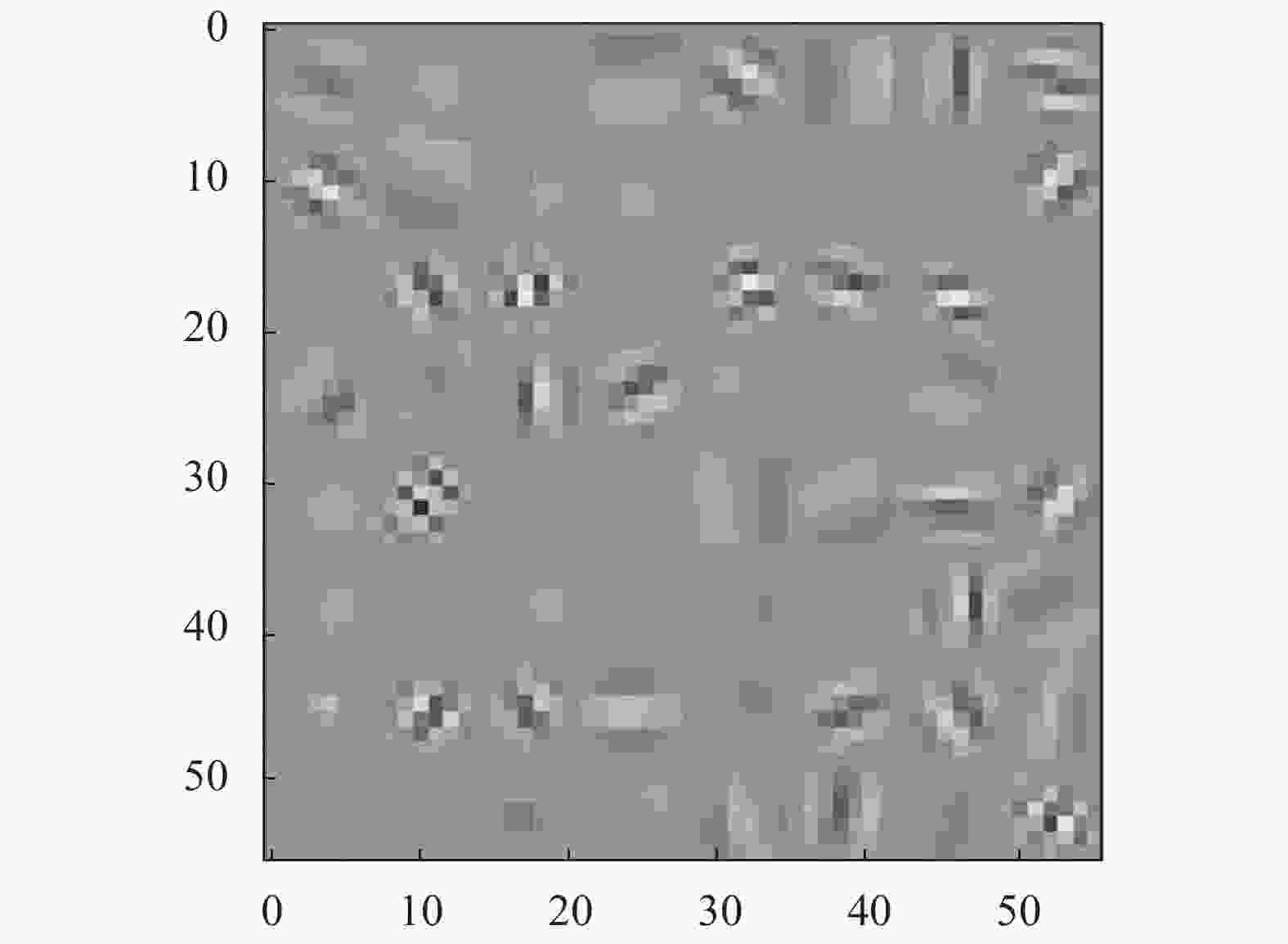
图 3 目标检测网络学习到的红外特征
Figure 3. IR features learned by object detection neural network
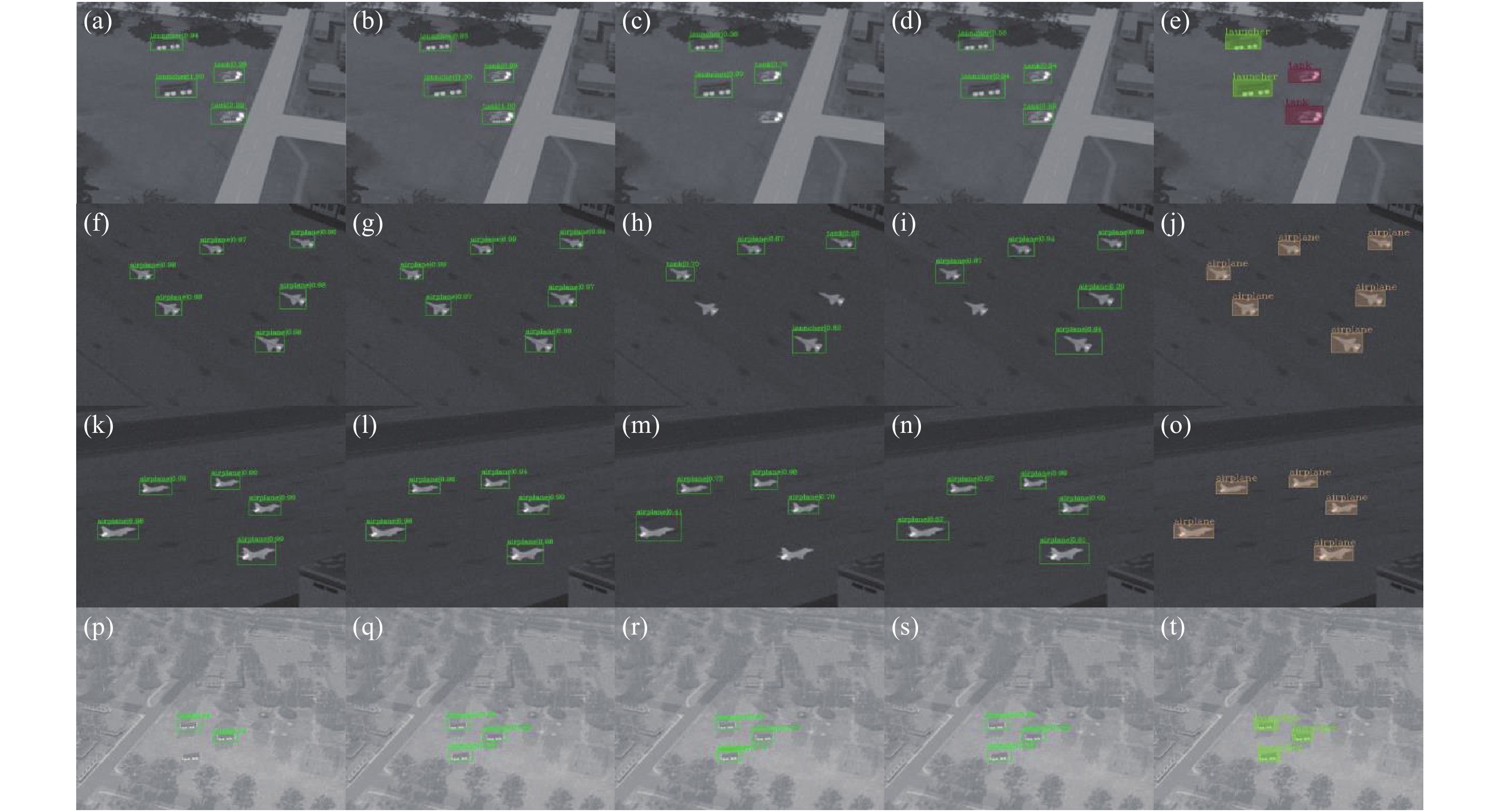
实验中部分代表性的检测结果如图4所示,其中每行为同一幅图片使用不同方法的检测结果,第一列至第四列分别为监督训练Faster R-CNN、半监督训练Faster R-CNN、监督训练YOLO-v3、半监督训练YOLO v3,最后一列为标注(Ground truth)。可以看出在第一行中,图4(c)监督训练YOLO-v3漏检了一个目标,相比之下图4(d)半监督训练的YOLO-v3正确补充了该目标;在第二行中,图4(h)监督训练的YOLO-v3漏检了两个目标,而图4(i)半监督训练YOLO-v3正确补充了一个目标;在第三行的结果中,图4(n)半监督训练YOLO-v3修正了图4(m)监督训练YOLO-v3的漏检;第四行中,图4(q)半监督训练Faster R-CNN修正了图4(p)监督训练Faster R-CNN的全部漏检。另外,文中发现Faster R-CNN对尺度变化的鲁棒性弱于YOLO-v3,而YOLO-v3在视角变化上的鲁棒性更弱,加入半监督训练后能够分别改善其短板:提高了Faster R-CNN对尺度变化的适应性和YOLO-v3对视角变化的鲁棒性。
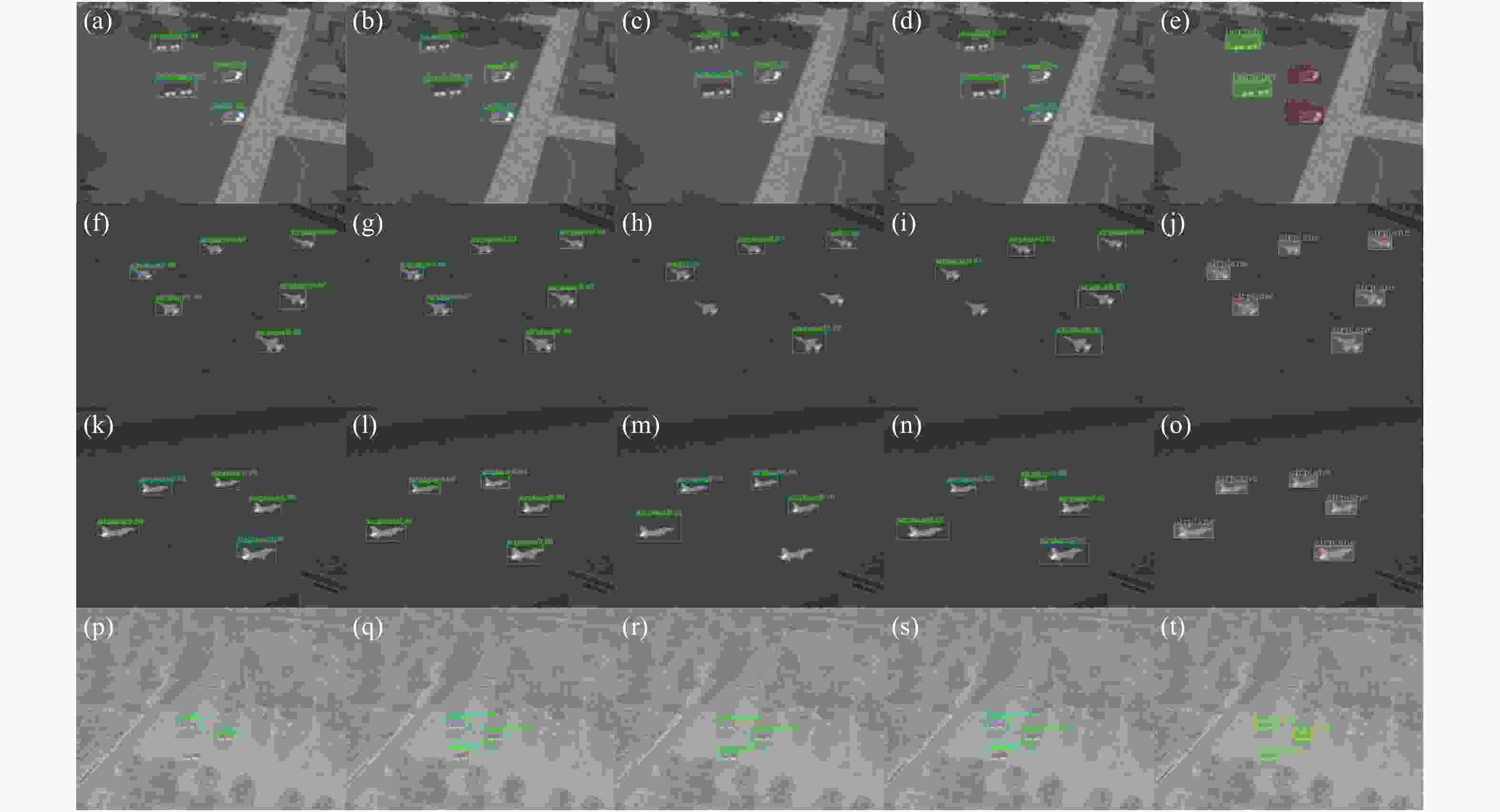
图 4 仅使用迁移学习与半监督迁移学习目标检测结果对比
Figure 4. Comparison of object detection with only transfer learning and with semi-supervised transfer learning
下面从定量的角度评估稀疏网络相比于稠密网络的参数压缩比例及其准确率的变化,主要用各个目标的检测准确率以及平均准确率(mAP)进行评价。
-
Faster R-CNN和YOLO-v3分别在红外图像训练集上训练60个和80个epochs,模型精度使用mAP (mean Average Precision)进行评价,并在包含150个目标的测试集上验证各个模型的mAP。各个目标检测模型的准确率如表3所示,其中Supervised transfer learning为仅仅使用有监督样本训练的模型,Semi-supervised transfer learning为使用额外无监督数据的半监督训练的模型。
表 3 红外图像数据集目标检测结果
Table 3. Object detection on infrared image dataset
Method Epochs Launcher Tank Airplane Battleship mAP Supervised transfer learning Faster R-CNN 60 0.946 0.995 0.965 0.980 0.972 YOLO-v3 80 0.964 0.848 0.919 0.979 0.927 Semi-supervised transfer learning Faster R-CNN 60 0.971 0.997 0.962 1.000 0.983 YOLO-v3 80 1.000 0.973 0.936 1.000 0.975 从表2中可以看出,无论对于Faster R-CNN还是YOLO-v3而言,半监督迁移学习模型的准确率都高于迁移学习模型,其在Faster R-CNN上实现了1.1%的少量提升,而在YOLO-v3上实现了4.8%的显著提升。关于YOLO-v3准确率提升高于Faster R-CNN,文中认为其原因在于原始的YOLO-v3对于视角变化的适应能力稍逊,而无标注样本的引入添加了不同视角的观测信息,修正了其观测视角不充分时的过拟合问题,从而提高了模型的泛化能力。无标注样本提升模型泛化能力的原理说明详见图1。
-
文中提出了一种红外目标检测网络的半监督迁移学习方法,主要用于提高目标检测网络在小样本红外数据集上的训练效率和泛化能力,提高深度学习方法在训练样本较少的红外目标检测场景当中的适应性。文中首先阐述了在标注样本较少时无标注样本对提高模型泛化能力、抑制过拟合方面的作用。在此基础上,提出了一种红外目标检测网络的半监督迁移学习方法。该方法首先使用大量的RGB图像对原始模型进程训练,获得预训练模型,随后使用少量的有标注红外图像和无标注红外图像对网络进行半监督学习调优,得到红外目标检测网络。为充分利用样本的分布信息,文中提出了一种特征相似度加权的伪监督损失函数,使用同一批次样本的预测结果相互作为监督信息,以充分利用无监督图像内相似目标的特征分布信息;为降低半监督训练的计算量,在伪监督损失函数的计算中,各目标仅考虑特征向量邻域范围内的预测结果作为伪标注。实验结果表明,该方法所训练的目标检测网络的测试准确率高于仅使用标注样本监督训练的网络,其在Faster R-CNN上实现了1.1%的提升,而在YOLO-v3上实现了4.8%的显著提升,验证了所提出方法的有效性。
An improved semi-supervised transfer learning method for infrared object detection neural network
-
摘要: 针对红外数据集规模小,标记样本少的特点,提出了一种红外目标检测网络的半监督迁移学习方法,主要用于提高目标检测网络在小样本红外数据集上的训练效率和泛化能力,提高深度学习模型在训练样本较少的红外目标检测等场景当中的适应性。文中首先阐述了在标注样本较少时无标注样本对提高模型泛化能力、抑制过拟合方面的作用。然后提出了红外目标检测网络的半监督迁移学习流程:在大量的RGB图像数据集中训练预训练模型,后使用少量的有标注红外图像和无标注红外图像对网络进行半监督学习调优。另外,文中提出了一种特征相似度加权的伪监督损失函数,使用同一批次样本的预测结果相互作为标注,以充分利用无标注图像内相似目标的特征分布信息;为降低半监督训练的计算量,在伪监督损失函数的计算中,各目标仅将其特征向量邻域范围内的预测目标作为伪标注。实验结果表明,文中方法所训练的目标检测网络的测试准确率高于监督迁移学习所获得的网络,其在Faster R-CNN上实现了1.1%的提升,而在YOLO-v3上实现了4.8%的显著提升,验证了所提出方法的有效性。Abstract: In view of the infrared datasets which has limited scale and few labeled samples, a semi-supervised transfer learning method was proposed for the training of infrared object detection neural network. It aimed at improving the training efficiency and generalization ability of object detection neural networks on infrared datasets with limited scale, and increasing the adaptability of deep learning models in scenarios with few training samples such as infrared object detection. Firstly, the ability of unlabeled samples in improving model generalization and suppressing overfitting under few labeled samples was described. Then, the process of semi-supervised transfer learning for infrared object detection neural network was proposed: a pre-trained model was trained on large scale RGB dataset, and next it was fine-tuned using a few labeled and unlabeled IR images. Moreover, a pseudo-supervised loss function with feature similarity weighting was proposed, where the predictions from same batch was used as labels to each other, thus making full use of the feature distribution of similar objects in unlabeled images. To reduce the computation of semi supervised learning, the pseudo-supervised loss of object was limited on the objects within the neighborhood of its feature vector. Experimental results show that the test accuracy of object detection neural network trained by proposed method is higher than that trained by supervised transfer learning, it achieves an improvement of 1.1% on Faster R-CNN and a significant improvement of 4.8% on YOLO-v3, which verifies the effectiveness of the proposed method.
-
图 2 红外目标检测网络的半监督迁移学习方法流程
Figure 2. Procedures of semi-supervised transfer learning of infrared object detection neural network
图 4 仅使用迁移学习与半监督迁移学习目标检测结果对比
Figure 4. Comparison of object detection with only transfer learning and with semi-supervised transfer learning
表 1 算法1: SSTL
Table 1. Algorithm 1: SSTL
Algorithm 1: SSTL Input: Detection neural network and the parameters $\{ {\theta ^{\rm{b}}},{\theta ^{{\rm{cls}}}},{\theta ^{{\rm{reg}}}}\} $ , RGB dataset${{\cal{D}}_{{\rm{RGB}}}}$ , labeled IR dataset${{\cal{D}}_I}$ , unlabeled IR dataset${{\cal{D}}_u}$ , weight of unsupervised loss${\alpha _{\max }}$ ,${t_{\max }}$ .Output: Trained neural network 1. Initialize parameters of neural network $\{ {\theta ^{\rm{b}}},{\theta ^{{\rm{cls}}}},{\theta ^{{\rm{reg}}}}\} $ , weight of unsupervised loss$\alpha = 0$ ;2. Pre-train $\{ {\theta ^{\rm{b}}},{\theta ^{{\rm{cls}}}},{\theta ^{{\rm{reg}}}}\} $ on RGB dataset${{\cal{D}}_{{\rm{RGB}}}}$ ;3. Adjust the number of output channels of classifier according to the number of categories of IR labels; 4. FOR Epoch t 5. FOR Each Batch 6. Sampling BatchSize training data form ${{\cal{D}}_I}$ and${{\cal{D}}_u}$ ;7. Getting the predictions ${\cal{P}}$ ,${\cal{C}}$ of batch images through forward propagation;8. Calculate the loss of predictions for supervised samples with Eq.(1); 9. For each ${{c}} \in {\cal{C}}$ , find the neighbourhood${\cal{N}}({{c}}) = \left\{ {{{{c}}_j},\left\| {{{f}}_{{c}}^{{\rm{cls}}} - {{f}}_{{{{c}}_j}}^{{\rm{cls}}}} \right\| < {R^{{\rm{cls}}}}} \right\}$ ;10. For each ${{p}} \in {\cal{P}}$ , find the neighbourhood${\cal{N}}({{p}}) = \left\{ {{{{p}}_j},\left\| {{{f}}_{{p}}^{{\rm{reg}}} - {{f}}_{{{{p}}_j}}^{{\rm{reg}}}} \right\| < {R^{{\rm{reg}}}}} \right\}$ ;11. Calculate the unsupervised loss of predictions through Eq.(7); 12. Calculate the gradient for semi-supervised loss Eq.(2); 13. Update $\{ {\theta ^{\rm{b}}},{\theta ^{{\rm{cls}}}},{\theta ^{{\rm{reg}}}}\} $ ;14. END FOR 15. Update the weight of unsupervised loss α with Eq.(9); 16. END FOR  下载: 导出CSV
表 2 红外仿真数据集
Table 2. Simulated infrared dataset
Classification Training Test Total Labeled Unlabeled Launcher 36 33 38 107 Tank 15 19 19 53 Airplane 42 41 42 125 Battleship 51 55 51 157 Total 144 148 150 442
下载: 导出CSV
表 3 红外图像数据集目标检测结果
Table 3. Object detection on infrared image dataset
Method Epochs Launcher Tank Airplane Battleship mAP Supervised transfer learning Faster R-CNN 60 0.946 0.995 0.965 0.980 0.972 YOLO-v3 80 0.964 0.848 0.919 0.979 0.927 Semi-supervised transfer learning Faster R-CNN 60 0.971 0.997 0.962 1.000 0.983 YOLO-v3 80 1.000 0.973 0.936 1.000 0.975
下载: 导出CSV
-
[1] Lienhart R, Maydt J. An extended set of Haar-like features for rapid object detection[C]//International Conference on Image Processing, 2002: 900-903. [2] Dalal N, Triggs B. Histograms of oriented gradients for human detection[C]//IEEE Computer Society Conference on Computer Vision & Pattern Recognition, 2005: 886-893. [3] Lowe D G. Distinctive image features from scale-invariant keypoints [J]. International Journal of Computer Vision, 2004, 60(2): 91-110. doi: 10.1023/B:VISI.0000029664.99615.94 [4] Bay H, Ess A, Tuytelaars T, et al. Speeded-up robust features [J]. Computer Vision and Image Understanding, 2008, 110(3): 346-359. doi: 10.1016/j.cviu.2007.09.014 [5] Li X, Wang L, Sung E. AdaBoost with SVM-based component classifiers [J]. Engineering Applications of Artificial Intelligence, 2008, 21(5): 785-795. doi: 10.1016/j.engappai.2007.07.001 [6] Felzenszwalb P F, Huttenlocher D P. Pictorial structures for object recognition [J]. International Journal of Computer Vision, 2005, 61(1): 55-79. doi: 10.1023/B:VISI.0000042934.15159.49 [7] Felzenszwalb P F, Girshick R B, McAllester D. Cascade object detection with deformable part models[C]//2010 IEEE Computer Society Conference on Computer Vision and Pattern Recognition, 2010: 2241-2248. [8] Felzenszwalb P F, Girshick R B, Mcallester D A. Visual object detection with deformable part models[C]//The Twenty-Third IEEE Conference on Computer Vision and Pattern Recognition, 2010. [9] Pratt L, Pratt L, Thrun S. Machine Learning - Special Issue on Inductive Transfer[M]. Netherland: Kluwer Academic Publishers, 1997. [10] Oquab M, Léon Bottou, Laptev I, et al. Learning and transferring mid-level image representations using convolutional neural networks[C]//IEEE Conference on Computer Vision & Pattern Recognition. IEEE, 2014. [11] Deng J, Dong W, Socher R, et al. ImageNet: A large-scale hierarchical image database[C]//IEEE Conference on Computer Vision & Pattern Recognition. IEEE, 2009. [12] Xie Bing, Duan Zhemin, Zheng Bin, Yin Yunhua. Research on UAV target recognition algorithm based on transfer learning SAE[J]. Infrared and Laser Engineering, 2018, 47(6): 0626001. (In Chinese) [13] Tang P, Wang X, Wang A, et al. Weakly supervised region proposal network and object detection[C]//Proceedings of the European Conference on Computer Vision. ECCV, 2018: 352–368. [14] Du L, Wei D, Li L, et al. SAR object detection network via semi-supervised learning [J]. Journal of Electronics and Information Technology, 2020, 42(1): 154-163. [15] Tang P, Ramaiah C, Wang Y, et al. Proposal learning for semi-supervised object detection[J]. arXiv preprint, arXiv, 2020: 2001.05086. [16] Ren S, He K, Girshick R, et al. Faster R-CNN: towards real-time object detection with region proposal networks [J]. IEEE Transactions on Pattern Analysis & Machine Intelligence, 2017, 39(6): 1137-1149. [17] Redmon J, Farhadi A. YOLOv3: an incremental improvement[J]. arXiv preprint, arXiv, 2018: 1804.02767. [18] Chen K, Wang J, Pang J, et al. Open MMLab detection toolbox and benchmark[J]. arXiv preprint, arXiv, 2019: 1906.07155. -

 点击查看大图
计量
- 文章访问数: 522
- HTML全文浏览量: 208
- PDF下载量: 101
- 被引次数: 0


