


 下载:
下载:


-
多飞行器地面试验中,精确估计每一个飞行器的运动是后续对多飞行器协同控制算法开发与制导控制系统性能评估等应用的基础。基于视觉的刚体运动估计是指根据给定的图像来估计物体的位置与姿态等参数,被广泛应用于运动恢复结构(SfM)[1]、视觉里程计(VO)[2]以及同时定位于建图(SLAM)[3]。
近年来,国内外学者对基于图像序列尤其是离散特征点的运动估计进行了大量的研究[4-6]。一般的,随着时间的推移基于特征点的多目标运动估计,尤其是无法对特征点进行全局跟踪时,估计结果会不可避免的产生累计误差,导致运动估计误差增大。因此,如何减少累积误差得到全局最优的估计结果,是获得准确可靠运动估计的重要内容。在近30年来,主要的解决方法包括滤波法与非线性优化法[7]。
对于滤波法,Brodia,Chandrashekhar等[8]利用序列图像结合迭代扩展卡尔曼滤波算法(IEKF)实现了目标运动参数的实时估计。仲小清等同样按参考文献[8]的方法结合基于交叉向量的运动参数测量原理为基础与串行卡尔曼滤波算法实现了运动估计,但实现方法需要加工高精度的激光合作目标[9]。
随着对于近十年来人们认识到BA(Bundle Adjustment)矩阵的稀疏特性,非线性优化算法逐渐被人们所重视,非线性优化方式主要包括光束法平差 [10]与位姿图(Pose Graph)优化[11-12]两种。MANOLIS等利用Bundle Adjustment方法求解计算机视觉中运动估计中的非线性最小二乘问题,分析了Bundle Adjustment矩阵的稀疏特性,并编制了通用稀疏Bundle Adjustment软件包[13]。Yasir等采用舍弃路标点的优化,只保留姿态之间的图边,使用位姿图对位姿估计的非线性最小二乘问题进行求解,并将图优化框架g2o引入非线性优化中,减小累计误差[14]。
为了实现对小尺寸飞行器地面试验中位姿的估计,文章第1节飞行器地面试验位姿估计系统构成及其工作原理进行描述;第2节提出了一种坐标系统一与飞行器位姿线性估计算法;第3节基于图模型对位姿估计结果进行非线性优化减小累积误差,最后通过实验对文中所提算法进行验证。
-
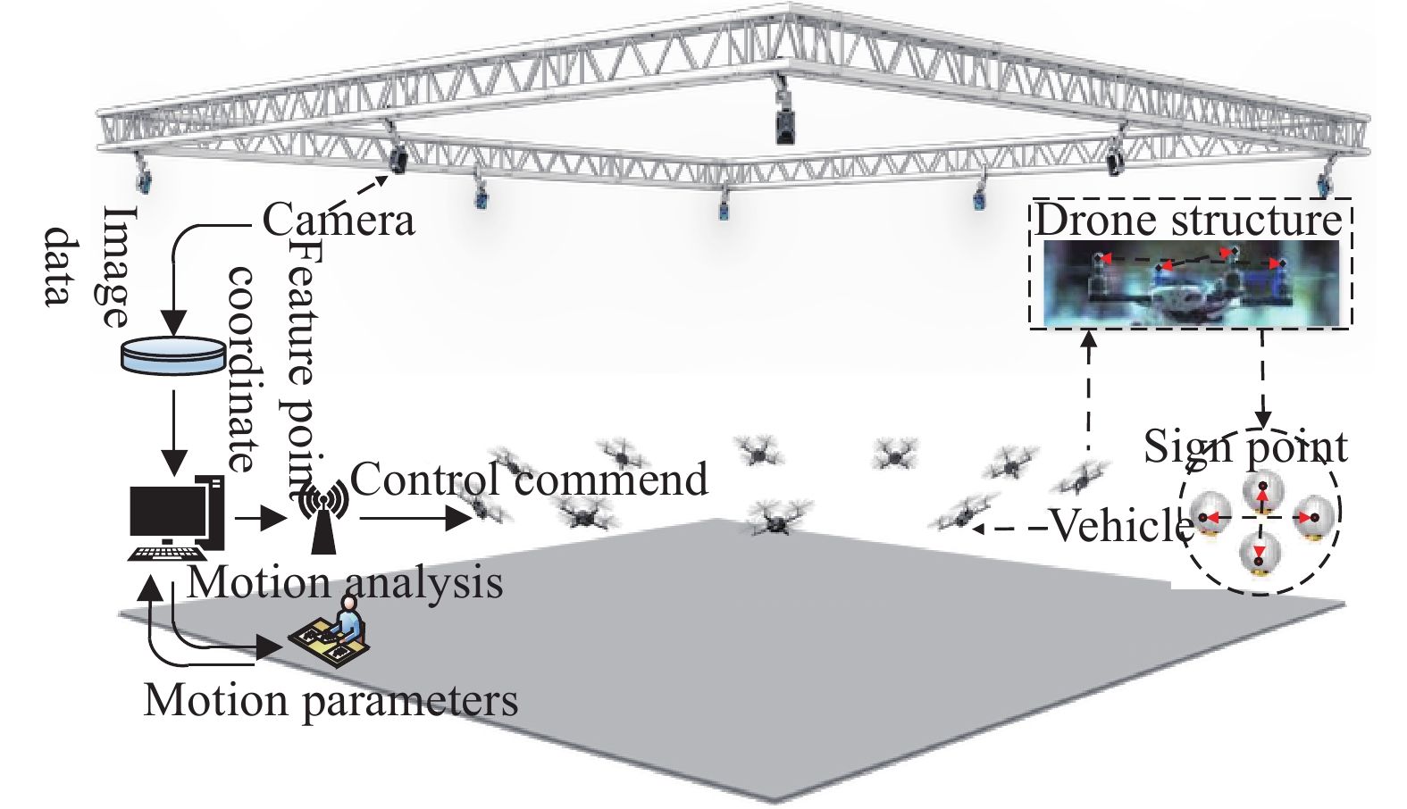
图1为飞行器地面试验位姿估计系统结构图。它主要由光学成像子系统、图像采集子系统、数据管理子系统、飞行器标记与照明子系统以及计算机等组成。飞行器标记与照明子系统由红外光源与具有红外反射涂层的靶标构成。图像采集子系统由CCD摄像机和图像采集卡等构成。进行位姿估计时,由图像采集系统采集运动估计空间中的飞行器图像,通过测量软件进行运动解算。

图 1 飞行器地面试验视觉定位系统原理图
Figure 1. Block diagram of vision position system of drones
-
该系统的基本工作原理为:飞行器位姿估计系统是由四台摄像机通过合理的布局实现对测量空间中的飞行器进行图像采集;利用球心成像点定位算法实现对于图像中合作靶标地点的定位[15];采用多摄像机三维定位算法实现飞行器上合作靶标点的三维定位[16];利用多目标跟踪算法实现对飞行器上合作靶标点的跟踪[17]。对于系统坐标系的统一采用中介坐标法确定飞行器发射坐标系与世界坐标系之间的转换关系。最后结合位姿估计算法对三维跟踪后的坐标点实现对飞行器位姿的高精度估计。
对于特征点的设计,采用被动式红外球形靶标,规避干扰,实现飞行器特征点的快速准确提取,提高系统的抗干扰能力。
-
如图2所示为飞行器位姿过程中的坐标系转换关系。为了实现对地面试验中飞行器位姿的高精度估计,即求解得到飞行器本体坐标系与发射坐标系之间的刚体变换
${T_{me}}$ 。需要首先标定得到世界坐标系与发射坐标系之间的变换${T_{ew}}$ ,然后依据公式(1)即可求解得到刚体变换: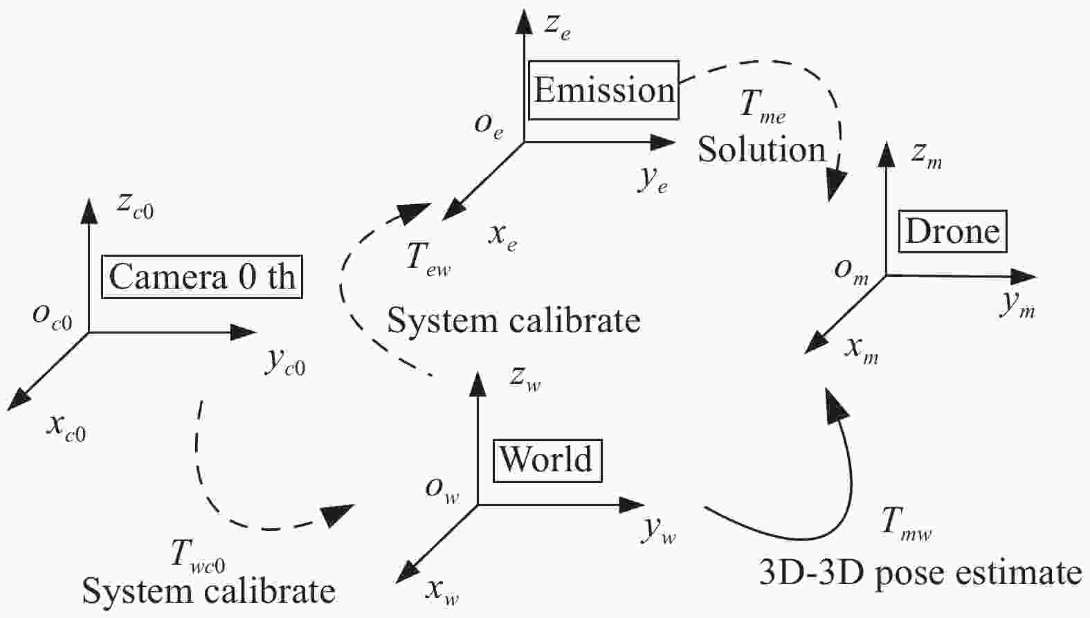
图 2 地面试验中飞行器视觉定位系统坐标系转换关系
Figure 2. Transform relationship of the frame between vehicle and vision positioning system in the ground test
$${T_{me}} = {T_{mw}} \bullet T_{ew}^{ - 1}$$ (1) 因此,若以第一个摄像机坐标系为世界坐标系,则对飞行器的位姿估计只需要首先实现世界坐标系与发射坐标系之间转换关系
${T_{ew}}$ 的求解,然后结合3D-3D运动估计算法求解得到飞行器相对于世界坐标系的刚体变换${T_{mw}}$ 。基于视觉的飞行器位姿估计方法归纳如下:
若设世界坐标系与第一个摄像机坐标系重合,则可根据多摄像机标定结果,将变换
${T_{eci}}$ 转换到世界坐标系下,并求得${T_{ew}}$ ,称为坐标系统一;根据3D-3D位姿估计算法求解得到飞行器在世界坐标系中的位姿
${T_{mw}}$ ,称为位姿估计。 -
如图3所示,设合作靶标点的质心为点
$o$ ,点1#与3#之间的方向向量为${{a}}$ ,点1#、2#与3#构成的平面法向量为$n$ 。若选择重心点$o$ 为坐标系原点,方向向量${{a}}$ 为$x$ 轴的方向,法向量${{n}}$ 方向为$z$ 轴方向,则根据向量叉乘可以求解得到${{c}} = {{a}} \times {{n}}$ ,取${{c}}$ 为$y$ 轴方向,建立飞行器本体坐标系,并将零位时刻的飞行器本体坐标系设为发射坐标系,即可实现对世界坐标系与发射坐标系之间的坐标系标定。现对其详细计算过程进行描述。
图 3 飞行器上合作靶标点的布局
Figure 3. Setup of sign point in the vehicle
根据多摄像机标定结果重建得到飞行器上合作靶标的世界坐标为
${p_i} = \left( {{x_i},{y_i},{z_i}} \right)$ ,$i = 1, \cdots ,M$ ,$M$ 表示合作靶标点的数目,则坐标原点为:$$o = \left( {{x_o},{y_o},{z_o}} \right) = \frac{1}{M}\left( {\sum\limits_{i = 1}^M {{x_i}} ,\sum\limits_{i = 1}^M {{y_i}} ,\sum\limits_{i = 1}^M {{z_i}} } \right)$$ (2) $x$ 轴方向向量为:$${{{n}}_x} = \left( {{x_3} - {x_1},{y_3} - {y_1},{z_3} - {z_1}} \right)$$ (3) $z$ 轴方向向量为:$${{{n}}_z} \cdot \left( {{x_i},{y_i},{z_i}} \right) = 0$$ (4) 式中:
$i = 1,2,3$ 。通过求解上述方程即可确定$z$ 轴方向向量。$y$ 轴方向向量由向量叉乘可以求解得到:$${{{n}}_y} = {{{n}}_x} \times {{{n}}_z}$$ (5) 因此,若定义如下两个矩阵:
$${{{D}}_w} = \left( {{n_x},{n_y},{n_z}} \right),{{{D}}_e} = \left[ {\begin{array}{*{20}{c}} 1&0&0 \\ 0&1&0 \\ 0&0&1 \end{array}} \right]$$ (6) 则世界坐标系到飞行器发射坐标系之间的旋转变换可以由以下公式获得:
$${{{R}}_{we}} = {{{D}}_w} \cdot {{D}}_e^{ - 1}$$ (7) 平移向量可以表示为:
$${{{t}}_{we}} = - {{R}}_{we}^{ - 1} \cdot {{o}}$$ (8) 最后为了使得坐标系原点在
$xoy$ 平面将平移向量${t_{we}}$ 平移如下位移量:$$\Delta {{t}} = \left( {0,0,{r_7}{x_1} + {r_8}{y_1} + {r_9}{z_1}} \right)$$ (9) 式中:
${r_7}$ 、${r_8}$ 与${r_9}$ 为矩阵${{{R}}_{we}}$ 的第三行元素。 -
对于飞行器上合作靶标点在世界坐标系中的坐标已经求解得到的位姿估计问题,文中采用一种向量交叉方法(Vector cross method, VC)进行求解。
设世界坐标系为
${O_w}{x_w}{y_w}{z_w}$ ,目标坐标系为${O_m}{x_m}{y_m}{z_m}$ ,若将飞行器位姿测量问题简化为刚体目标位姿测量,则飞行器位姿估计问题可等价为求解目标坐标系与测量坐标系之间的转换关系${{{C}}_{mw}}$ ,其中${{C}}_{mw}h$ 包括旋转矩阵与平移向量${{{R}}_{mw}}$ 和${{{T}}_{mw}}$ 。若已知合作靶标在目标体坐标系下坐标为
${{{P}}_{mi}} = {\left( {{x_{mi}},{y_{mi}},{z_{mi}}} \right)\rm{^T}}$ ,在世界坐标系中的坐标为${{{P}}_{wi}} = {\left( {{x_{wi}},{y_{wi}},{z_{wi}}} \right)\rm{^T}}$ ,$i = 1,2,3,4$ ,则根据刚体旋动理论,位姿求解模型可以表示为:$${{{P}}_{wi}} = {{{R}}_{wm}}{{{P}}_{mi}} + {{{T}}_{mw0}}$$ (10) 定义
${{{A}}_{wj}} = {{\left( {{{{P}}_{w\left( {j + 2} \right)}} - {{{P}}_{wj}}} \right)} / {\left| {{{{P}}_{w\left( {j + 2} \right)}} - {{{P}}_{wj}}} \right|}}{\kern 1pt} {\kern 1pt} $ ,显然$\left| {{{{P}}_{w\left( {j + 2} \right)}} - {{{P}}_{wj}}} \right| \ne {\rm{0}}$ ,${\kern 1pt} {\kern 1pt} {\kern 1pt} {\kern 1pt} {\kern 1pt} \left( {j = 1,2} \right)$ ;进一步定义${{{B}}_w} ={{{A}}_{w1}} \times $ $ {{{A}}_{w2}} / \left| {{{A}}_{w1}} \times {{{A}}_{w2}} \right|$ ,且$\left| {{{\bf{A}}_{w1}} \times {{\bf{A}}_{w2}}} \right| \ne {\rm{0}}$ ,因此可以构造一个新的矩阵${{{D}}_w}$ [18]:$${{{D}}_w} = \left( {{{{A}}_{w1}},{{{A}}_{w2}},{{{B}}_w}} \right)$$ (11) 对于目标坐标系,相应的也可以构造一个矩阵
${{{D}}_m}$ 。若规定则${{{R}}_{wm}}$ 为世界坐标系与目标坐标系之间的旋转变化矩阵,则:$${{{D}}_w} = {{{R}}_{wm}}{{{D}}_m}$$ (12) 根据
${{{D}}_w}$ 和${{{D}}_m}$ 的构造方式,以及刚体上两向量不共线的条件可知:${{{D}}_w}$ 和${{{D}}_m}$ 均满秩。因此,可以通过公式(5)求取目标坐标系相对于测量坐标系之间的旋转矩阵${R_{mw}}$ :$${{{R}}_{mw}} = {\left( {{{{D}}_w} \cdot {{D}}_m^{ - 1}} \right)^{ - 1}}$$ (13) 对于位置向量
${{{T}}_{mwo}}$ ,可以分别取${P_1}$ ,${P_3}$ 特征点所在直线与${P_2}$ ,${P_4}$ 特征点所在直线的交点在目标坐标系下的坐标${X_m}$ 和在测量坐标系中的坐标${X_w}$ ,根据公式(10)可求得:$$ {{{T}}_{mw0}} = {{{X}}_w} - {{{R}}_{wm}}{{{X}}_m} $$ (14) -
本节根据飞行器地面试验中位姿估计的特点,建立了位姿估计图模型,并对问题进行了求解。
-
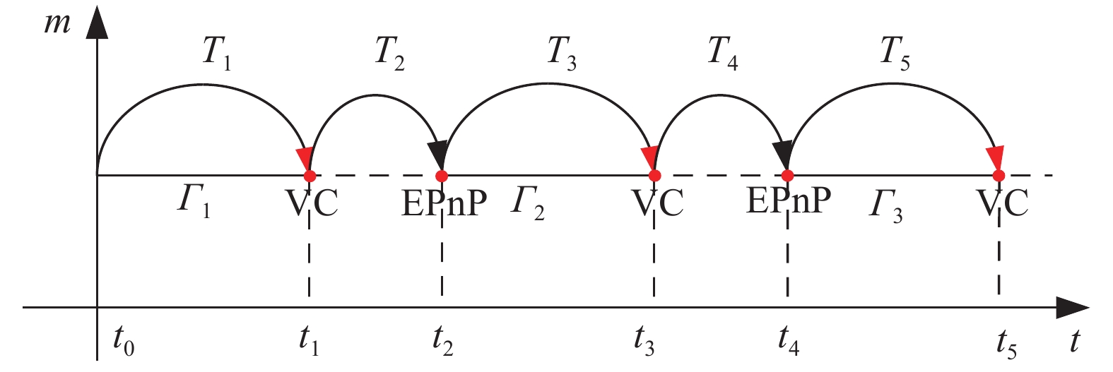
由于飞行器的进出视场、遮挡等原因,导致多目标跟踪算法获得的合作靶标点的轨迹不连续[17]。如图4所示,在每一数据关联准确的轨迹段
${\varGamma _i}$ 内,直接线性位姿估计算法的局部估计结果为轨迹段内的最大后验估计值${T_{2k + 1}}$ 。为了实现飞行器位姿的全局估计目的,需要进行相邻轨迹段之间相对位姿${T_{2k + 2}}$ 分别进行估计,然后对位姿结果进行累乘。此时绝对位姿估计误差的主要来源为累乘所导致的累积误差。如公式(15)所示:$${{{T}}_N} = \prod\limits_{n = 0}^N {\left( {{T_n} + \Delta {T_n}} \right)} $$ (15) 式中:T表示飞行器的刚体变换矩阵;N表示飞行器在测量期间同一靶标点所产生的轨迹段数;ΔT表示每段轨迹所产生的位姿估计误差。

图 4 飞行器定位误差累计示意图
Figure 4. Accumulated schematic diagram of vehicle positioning error
-
为了实现对飞行器位姿估计结果进行非线性优化减小累积误差,本节根据飞行器地面试验中位姿估计系统的特点,将位姿估计的非线性问题建模为一个图优化模型,如图5所示,其中主要包括位姿节点、状态转移边、特征测量边以及特征点。且在各自轨迹段
${\varGamma _i}$ 内合作靶标点数据已关联,因此其具有解析解,不需要进行非线性优化,但对于轨迹之间合作靶标点无数据关联关系,为了减小误差,首先利用EPnP(Efficient Perspective-n-Point)算法[19]根据合作靶标点在飞行器发射坐标系下的坐标求解得到下一轨迹相对于初始零位的位姿关系初始值,并结合回环检测算法对飞行器位置进行重定位[20],最后将位姿估计问题建立为一个非线性最小二乘问题,利用通用图优化库(g2o)进行求解。
图 5 做圆弧运动的飞行器位姿估计图优化模型
Figure 5. Graph optimal model of vehicle pose estimation with a circle trajectory motion
根据上述图表示的飞行器位姿估计问题构建一个非线性最小二乘问题。其目标函数可以表示为:
$${{{\xi }}^*} = \mathop {\arg \min }\limits_{{\xi }} \frac{1}{2}\sum\limits_{i,j \in \varepsilon } {e_{ij}{\rm{^T}}{{\Sigma }}_{ij}^{ - 1}{e_{ij}}} $$ (16) 式中:
${e_{ij}} = \ln {\left( {{{T}}_{ij}^{ - 1}{{T}}_i^{ - 1}{{{T}}_j}} \right)^ \vee }$ ,${{{T}}_i}$ 为摄像机在飞行器本体坐标系中的位姿R;t的李群表示;${{\Sigma }}_{ij}^{ - 1}$ 表示误差项的信息矩阵;${{{T}}_{ij}}$ 表示向量位姿节点之间的位姿关系的李群表示;$j = N$ 表示摄像机采集的总帧数。 -
位姿估计的图优化是指将位姿估计优化问题转换为图的形式,其中一个图由若干个顶点(Vertex)以及连接顶点之间的边(Edge)所组成。其中顶点表示优化变量,边表示误差项。根据构建的飞行器地面试验位姿估计图优化模型,误差边可以表示为:
$${\hat e_{ij}} = \ln {\left( {{{T}}_{ij}^{ - 1}{{T}}_i^{ - 1}\exp {{\left( { - \delta {{{\xi }}_i}} \right)}^ \wedge }\exp \left( {\delta {{\xi }}_j^ \wedge } \right){{{T}}_j}} \right)^ \vee },$$ (17) 又根据伴随的性质可知[12]:
$$\begin{split} {{\hat e}_{ij}} =\;&\ln {\left( {{{T}}_{ij}^{ - 1}{{T}}_i^{ - 1}\exp {{\left( { - \delta {{{\xi }}_i}} \right)}^ \wedge }\exp \left( {\delta {{\xi }}_j^ \wedge } \right){{{T}}_j}} \right)^ \vee} \approx \\ & \ln {\left( {{{T}}_{ij}^{ - 1}{{T}}_i^{ - 1}{{{T}}_j}\left[ {{{I}} - {{\left( {Ad\left( {{{T}}_j^{ - 1}} \right)\delta {{{\xi }}_i}} \right)}^ \wedge } + {{\left( {Ad\left( {{{T}}_j^{ - 1}} \right)\delta {{{\xi }}_j}} \right)}^ \wedge }} \right]} \right)^ \vee }\approx \\ & {e_{ij}} + \frac{{\partial {e_{ij}}}}{{\partial \delta {{{\xi }}_i}}}\delta {{{\xi }}_i} + \frac{{\partial {e_{ij}}}}{{\partial \delta {{{\xi }}_j}}}\delta {{{\xi }}_j}\\[-15pt] \end{split} $$ (18) 根据李代数求导法则可得:
$$\left\{ \begin{aligned} & \frac{{\partial {e_{ij}}}}{{\partial \delta {{\bf{\xi }}_i}}} = - J_r^{ - 1}\left( {{e_{ij}}} \right)Ad\left( {{{T}}_j^{ - 1}} \right) \\ &\frac{{\partial {e_{ij}}}}{{\partial \delta {{\bf{\xi }}_j}}} = - J_r^{ - 1}\left( {{e_{ij}}} \right)Ad\left( {{{T}}_j^{ - 1}} \right) \end{aligned} \right.$$ (19) 取
${J_r}$ 的近似:$$J_r^{ - 1}\left( {{e_{ij}}} \right) \approx I + \frac{1}{2}\left[ {\begin{array}{*{20}{c}} {\phi _e^ \wedge }&{\rho _e^ \wedge } \\ {\bf{0}}&{\phi _e^ \wedge } \end{array}} \right]$$ (20) 最后, 利用通用图优化库(g2o)即可实现对上述最小二乘问题进行求解,从而得到非线性优化后的位姿估计结果。
-
本小节分别通过计算机仿真分析与实际图像估计实验对文中提出的飞行器地面试验中的位姿估计算法进行精度与鲁棒性分析以及可行性验证。
-
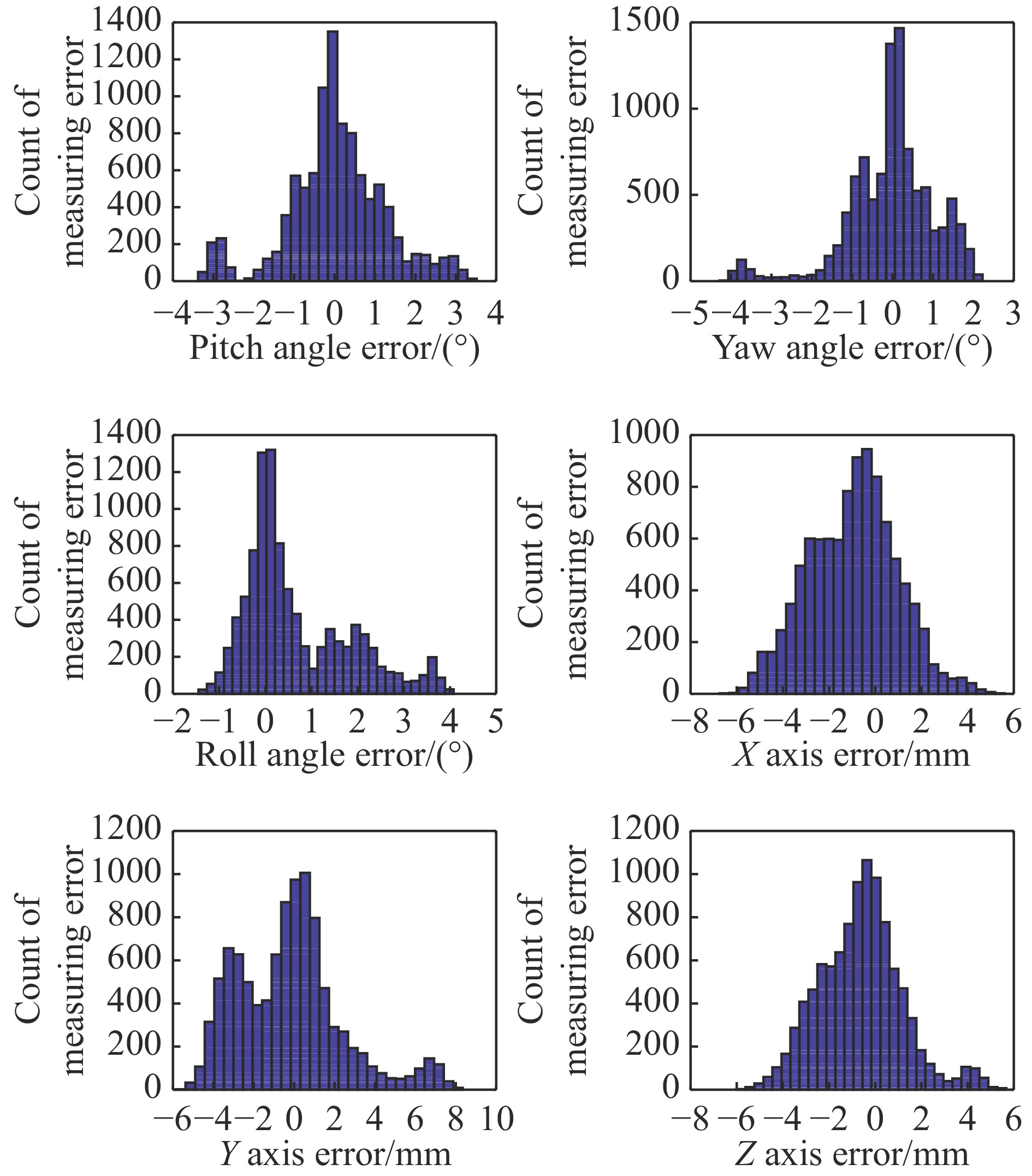
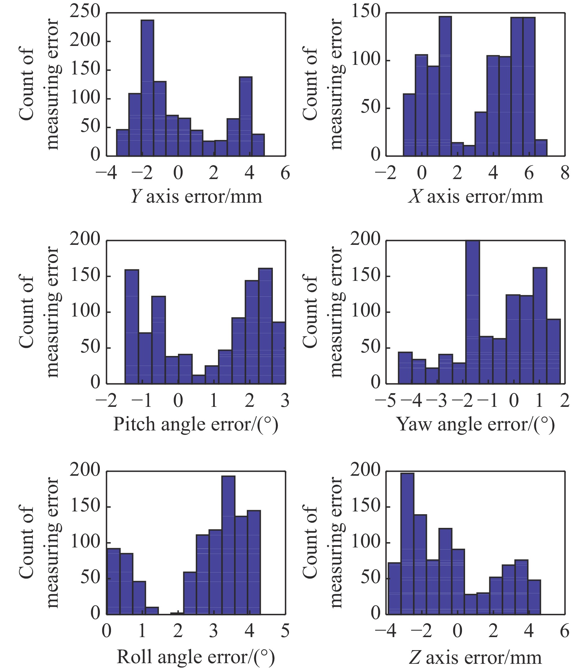
为了实现对文中提出算法的精度进行验证,假设飞行器尺寸为400 mm(即合作靶标之间的最大距离小于等于400 mm),三维定位误差采用均值0,方差3 mm的高斯白噪声模拟,姿态角度变化在0~30°之间按照正弦规律变化,位移变化在0~1 000 mm之间均匀变化。将飞行器轨迹分成4小段,然后利用直接线性位姿估计算法对每一段单独对位姿进行估计,利用基于图模型的非线性优化算法对直接线性位姿估计算法的求解结果进行优化,并最终将测量结果转换到飞行器发射坐标系中。实验时进行1 000次仿真实验,并统计误差直方图如图6~7所示。

图 6 直接线性位姿估计算法误差统计
Figure 6. Error statistical of linear posture estimation algorithm
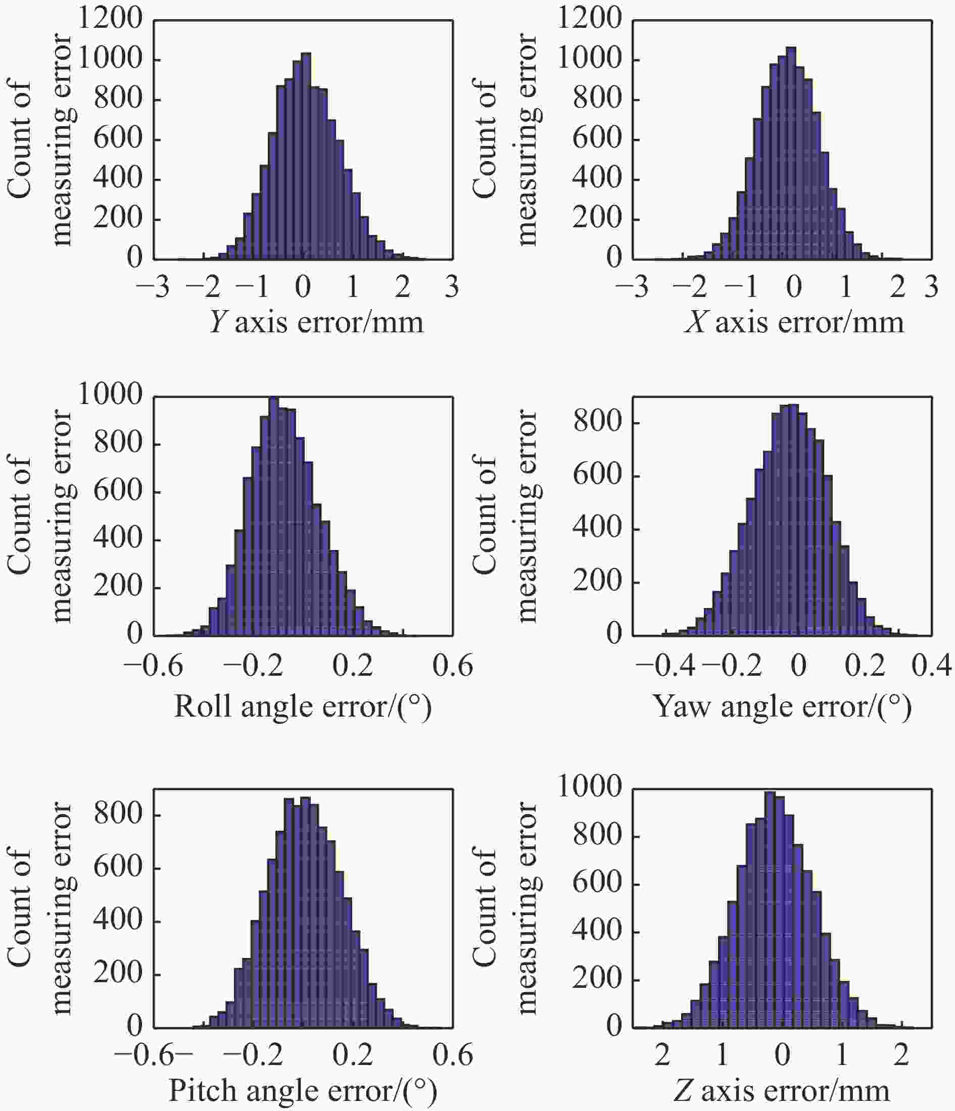
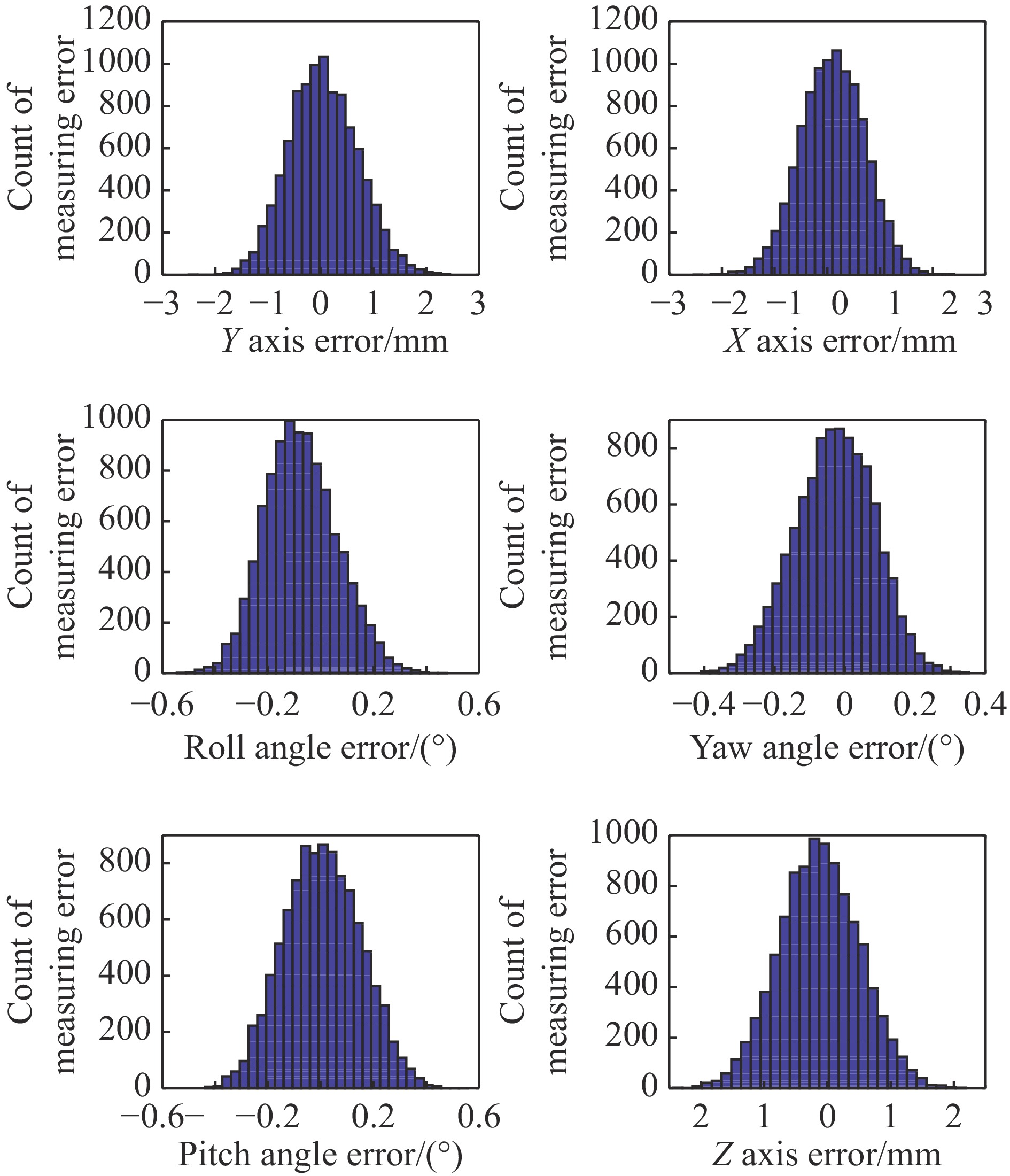
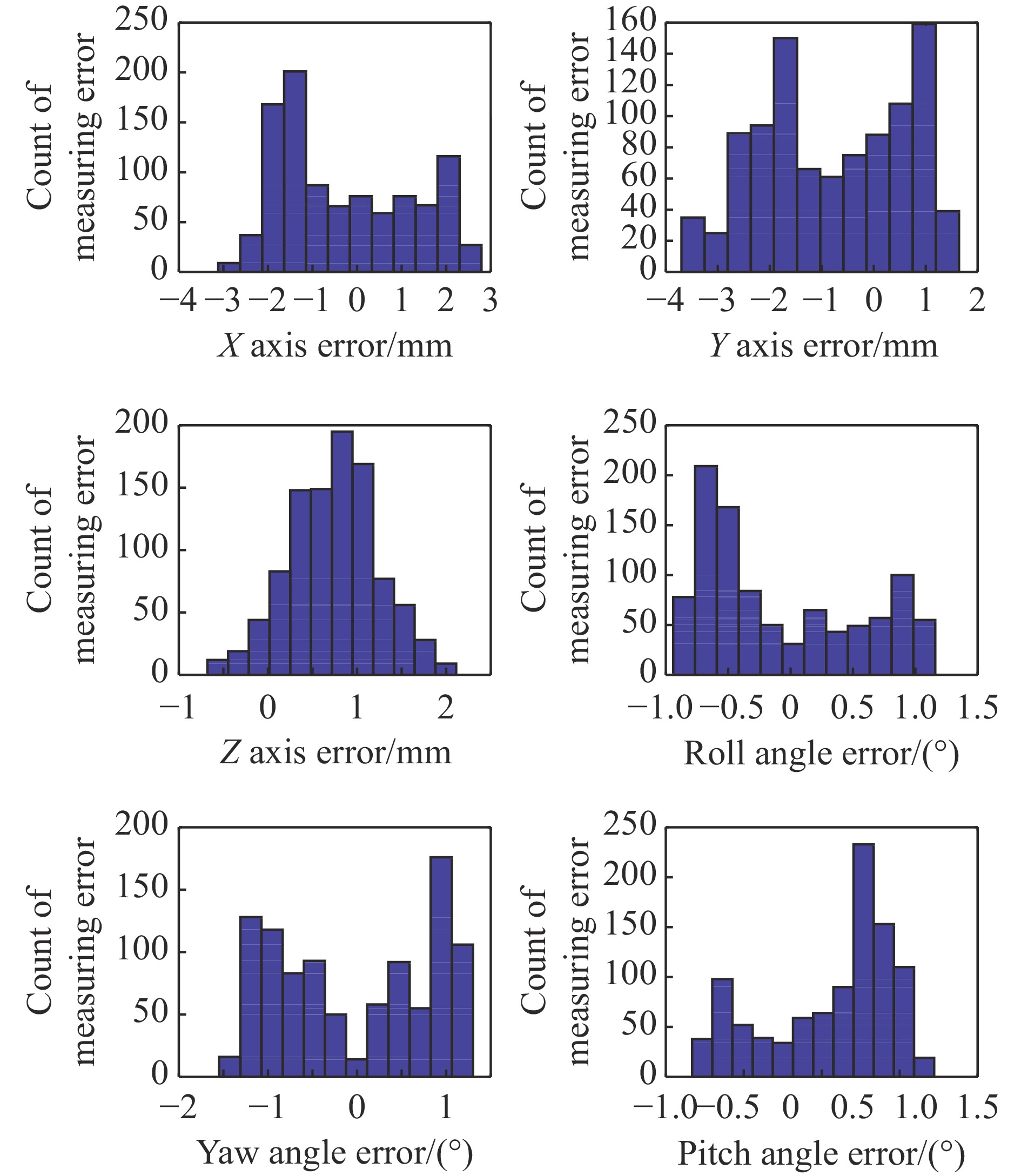
图 7 采用非线性优化后的位姿估计算法误差统计
Figure 7. Error statistical of nonlinear optimal posture estimation algorithm
(1)文中提出的飞行器位姿线性定位算法对姿态的定位精度为4°(3σ),对位置的定位精度为6 mm(3σ),这主要是由于轨迹片段引起位姿估计误差累积所导致的;
(2)文中提出的非线性优化算法对飞行器姿态定位精度在0.5°(3σ),对位置的定位精度在3 mm(3σ)以内,且可以看出非线性优化算法明显减小了累计误差且基本符合高斯分布,说明在无坐标系转换误差的条件下,非线性优化后的误差来源主要是合作靶标点的三维定位误差;
(3)非线性优化后偏航角的误差小于其他两个姿态角的原因是由于姿态角的测量基线略长于其他两个姿态角所导致的。
-
然后,统计了不同三维定位误差条件下直接线性位姿估计算法与基于图模型的非线性优化算法误差的大小。其中误差等级为均值为0,方差从0~5 mm变换的高斯白噪声。飞行器角度变化为30°,位移变化为0 mm。分别利用文中提出的线性位姿解算算法以及非线性优化算法进行位姿估计,并统计每一误差等级下的误差均值。误差统计结果如图8所示。
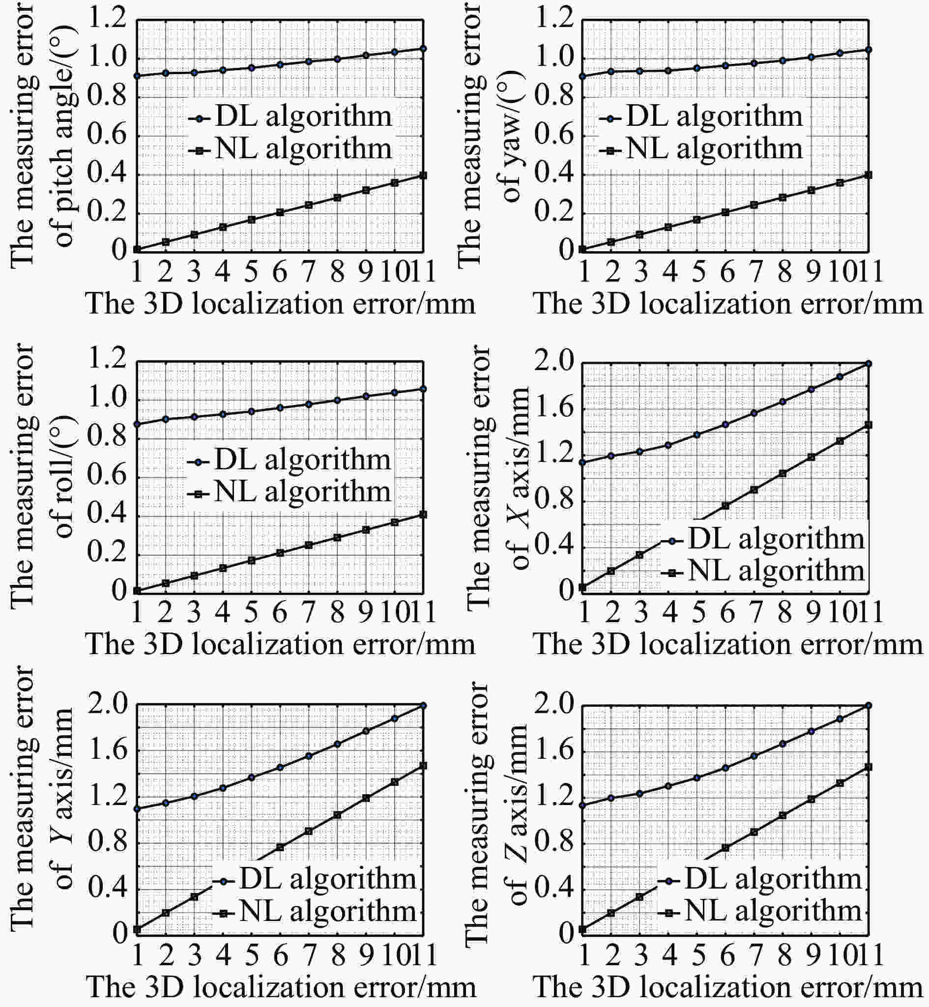
图 8 飞行器非线性优化前后位姿估计结果相对3D定位误差的均方值分布
Figure 8. Mean error distribution of relative 3D localization error of estimation algorithm before and after nonlinear optimization
根据图8误差统计结果可知:
(1)两种算法对飞行器的位姿估计误差都随着合作靶标点的三维定位误差增大而增大;
(2)基于图模型的非线性优化算法的位姿估计精度虽然也随着合作靶标点的定位误差增大,但其大小明显小于线线解法。这说明文中提出的非线性优化算法最大限度的利用了所有采集时刻的合作靶标定位坐标进行优化计算;
(3)直接线性位姿估计算法在三维定位误差较小时,其位姿估计误差明显大于非线性优化算法,随着三维定位误差的增大,两者的误差增长斜率趋近于一致,这说明此时,累加误差已不再是主要误差来源,三维定位误差转而称为了主要误差源。
-
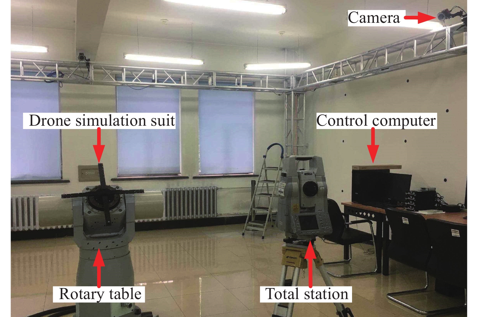
为了验证文中提出的基于图模型的位姿估计非线性优化算法的性能,将飞行器模拟装置固定在转台上,通过转台运动来模拟飞行器的运动,其中飞行器运动姿态角按
$y = 30\sin \left( {0.2\pi t} \right)$ 给定,并将视觉位姿估计系统的结果与姿态给定装置的给定值进行比较。其中飞行器的尺寸约为400 mm,采用的摄像机为:IO Industry Canada, Flare 4M140, 传感器尺寸为:2 048 × 2 048 pixel,像元大小为:5.5 μm. 镜头焦距为f = 12.5 mm。测量系统的标定误差为2.9 mm,为了模拟跟踪算法的轨迹不连续问题,将轨迹分成4段,其中图9为算法评估系统图。图10、11分别为非线性优化前后飞行器的位姿估计误差统计直方图。
图 9 实际位姿估计算法测试系统
Figure 9. Actual posture estimation accuracy verification experimental device

图 10 直接线性算法姿态估计结果
Figure 10. Result of pose estimate based on linear algorithm
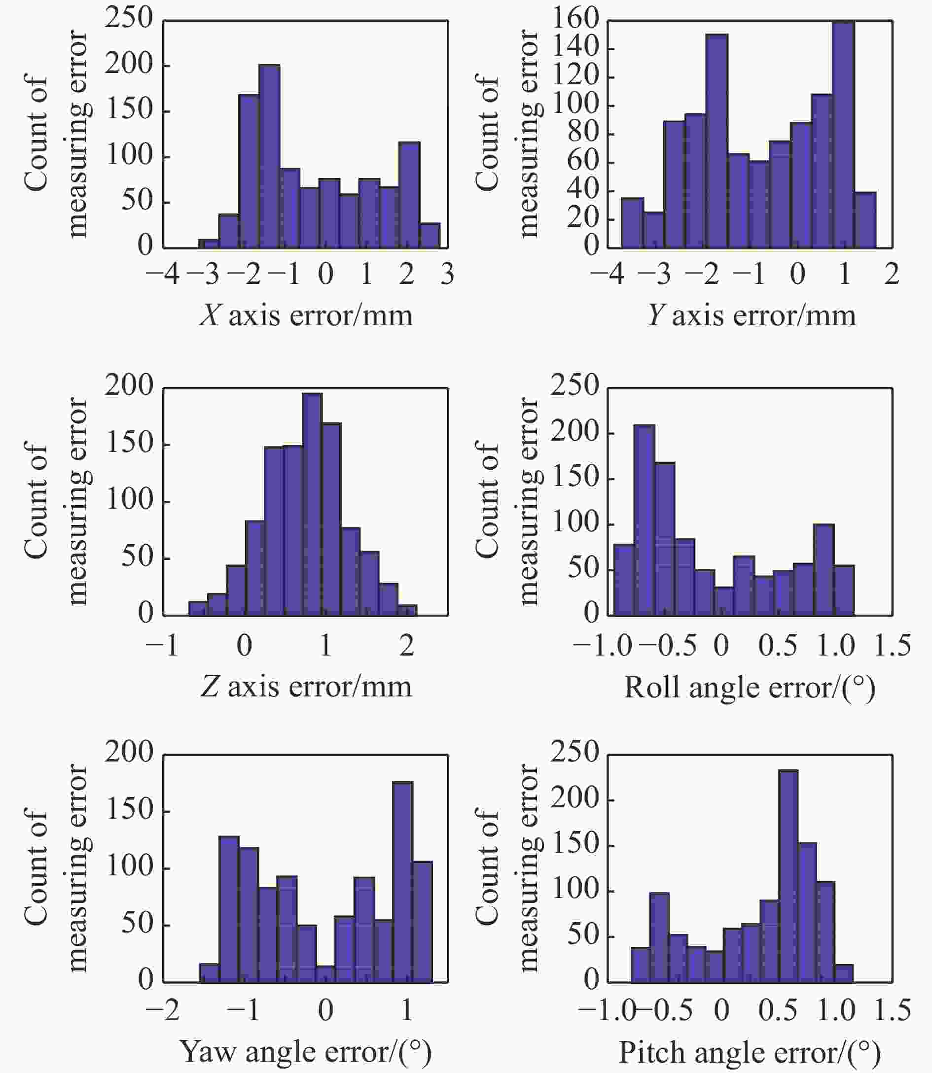
图 11 基于图模型的非线性位姿估计误差统计直方图
Figure 11. Result of pose estimate based on nonlinear algorithm
(1)基于直接线性位姿估计算法精度为4°(3σ),位置估计算法精度为6 mm(3σ),基于图模型的非线性算法估计得到的实际绝对姿态误差小于1.3°(3σ),位置误差小于4 mm(3σ);
(2)相比于基于图模型的非线性优化算法,基于直线的位姿估计算法的误差分布均偏离0位,这是因为采用初始帧的测量结果作为零位,将零位与理想值之间的误差引入到后续位姿估计结果中,表现为波动中心不一致,且不为零的情况;
(3)相比于直接线性算法,非线性优化算法估计得到的位姿参数中的累积误差大大减小,这说明文中提出的非线性优化算法大大减小了累计误差项。
-
文中根据飞行器地面试验中对其制导控制系统性能评估对运动参数估计精度的要求,提出了一种基于图模型的位姿高精度估计方法,并建立了一套飞行器位姿估计测量系统,介绍了其工作原理。研究了基于图模型的飞行器非线性优化方法。最后,分别通过仿真分析与实际位姿估计实验对文中提出算法的性能进行了分析。实验结果表明:在飞行器尺寸为400 mm,测量范围为6 000 mm×6 000 mm×3 000 mm,标定精度为2.9 mm时,姿态估计精度可达1.3°(3σ),位置定位精度可达4 mm(3σ)。基本满足对于惯性导航精度在1.5°左右的小尺寸飞行器制导控制系统性能长时间评估的要求。
需要指出的是,因为实际实验过程中需要对系统进行全局统一,这势必会引入坐标系统一误差到最后的测量误差中,因此文中求解得到的位姿估计精度还可以通过高精度的系统标定设备进一步提高,且根据仿真结果可知其姿态估计理论值可达0.5°(3σ),位姿估计精度可达3 mm(3σ)。
Research on posture estimation method of small-size vehicle in the ground test based on the graph optimal model
-
摘要: 在多飞行器地面试验位姿估计中,由于跟踪算法导致的跟踪轨迹不连续会使得位姿估计产生累积误差,为了实现位姿的精确估计,提出了一种基于图模型的全局位姿估计非线性优化方法。首先,建立了一个飞行器地面视觉位姿估计系统。然后根据飞行器上特征点的数目提出了一种向量交叉式的飞行器位姿解算方法,求解得到数据已关联飞行器位姿估计值。利用中介坐标系法求解得到轨迹段初始位姿节点在测量坐标系下的值,最后,在图模型基础上下,对整个量测过程中飞行器的位姿估计结果进行非线性全局优化减小线性算法的累积误差,并通过仿真与实际实验对飞行器位姿估计算法的可行性与精度进行验证。实验结果表明:在测量范围为6 000 mm×6 000 mm×3 000 mm的范围内,飞行器尺寸约为400 mm,特征点三维定位精度为2.9 mm的条件下,基于非线性优化的飞行器位姿估计算法的理论精度分别可达0.5° (3σ)与3 mm (3σ),实际绝对测量精度分别可达1.3°(3σ)与4 mm (3σ),基本满足地面试验对多飞行器编队算法开发以及制导控制系统性能长时间评估稳定可靠、精度高、抗干扰能力强等要求。Abstract: In the ground test of multi-vehicle, the global motion estimation method based on graph optimization model was proposed in order to reduce the cumulative error of posture estimation due to the discontinuity of tracking trajectory caused by tracking algorithm. Firstly, a ground test vision motion estimation system for vehicle was established. Then, according to the number of feature points on the vehicle, a vector crossover method was proposed to solve the position of vehicle posture, and the estimation value of vehicle posture with good data correlation was obtained. The intermediate coordinate system method was used to solve the value of the initial position node of the track segment under the measuring coordinate system, and finally, under the framework of graph optimization theory, the nonlinear global optimization of the motion estimation results of the vehicle during the whole measurement process was carried out to reduce the cumulative error of the linear algorithm, and the feasibility and precision of the vehicle motion estimation algorithm were verified by simulation and practical experiments. The experimental results show that the accuracy of the proposed vehicle attitude estimation algorithm can reach 0.5° (3σ) and 3 mm (3σ) respectively, and the actual absolute measurement accuracy can reach 1.3° (3σ) and 4 mm (3σ) respectively, the size of the vehicle is 400 mm in the range of the measuring range of 6 000 mm×6 000 mm×3 000 mm and the three-dimensional positioning accuracy of the feature points is 2.9 mm. It basically meets the requirements of ground test for the development of multi-vehicle formation algorithm and the performance evaluation of guidance control system, stable and reliable, high precision and strong anti-jamming ability.
-
Key words:
- computer vision /
- pose estimate /
- graph theory /
- system calibration /
- vector cross
-
图 2 地面试验中飞行器视觉定位系统坐标系转换关系
Figure 2. Transform relationship of the frame between vehicle and vision positioning system in the ground test
图 5 做圆弧运动的飞行器位姿估计图优化模型
Figure 5. Graph optimal model of vehicle pose estimation with a circle trajectory motion
图 7 采用非线性优化后的位姿估计算法误差统计
Figure 7. Error statistical of nonlinear optimal posture estimation algorithm
图 8 飞行器非线性优化前后位姿估计结果相对3D定位误差的均方值分布
Figure 8. Mean error distribution of relative 3D localization error of estimation algorithm before and after nonlinear optimization
图 9 实际位姿估计算法测试系统
Figure 9. Actual posture estimation accuracy verification experimental device
-
[1] Schonberger J L, Frahm J M. Structure-from-motion revisited[C]// Proceedings of the IEEE Conference on Computer Vision and Pattern Recognition. 2016: 4104-4113. [2] Scaramuzza D , Fraundorfer F. Visual odometry tutorial [J]. IEEE Robotics & Automation Magazine, 2011, 18(4): 80−92. [3] Cadena, Cesar, Carlone, et al. Past, present, and future of simultaneous localization and mapping: Toward the robust-perception age [J]. IEEE Transactions on Robotics, 2016, 32(6): 1309−1332. doi: 10.1109/TRO.2016.2624754 [4] John Weng, Narendra Ahuja, Thomas S H. Learning recognition and segmentation using the cresceptron [J]. International Journal of Computer Vision, 1997, 25(2): 109−143. doi: 10.1023/A:1007967800668 [5] Hartley R I. In defense of the eight-point algorithm [J]. IEEE Transactions on Pattern Analysis and Machine Intelligence, 1997, 19(6): 580−593. doi: 10.1109/34.601246 [6] Pomerleau F, Colas F, Siegwart R. A review of point cloud registration algorithms for mobile robotics [J]. Foundations and Trends in Robotics, 2015, 4(1): 1−104. doi: 10.1561/2300000035 [7] Gao Xiang, Zhang Tao. The 14 Lecture of Visual SLAM: From Theory to Practical[M].Beijing: Electronic Industry Press, 2017. (in Chinese) [8] Broida T J, Chandrashekhar S, Chellappa R. Recursive 3-D motion estimation from a monocular image sequence [J]. IEEE Transactions on Aerospace and Electronic Systems, 1990, 26(4): 639−656. doi: 10.1109/7.55557 [9] Huo Ju, Zhong Xiaoqing, Yang Ming. Motion Estimation of a vehicle using sequential recursive algorithm from images [J]. Journal of Astronautics, 2010, 31(2): 361−368. [10] Triggs B, McLauchlan P F, Hartley R I, et al. Bundle adjustment—a modern synthesis[C]//International Workshop on Vision Algorithms, 1999: 298-372. [11] Dubbelman G, Browning B. Cop-slam: Closed-form online pose-chain optimization for visual slam [J]. IEEE Transactions on Robotics, 2015, 31(1): 1194−1213. [12] Lee D, Myung H. Solution to the slam problem in low dynamic environments using a pose graph and an RGB-D sensor [J]. Sensors, 2014, 14(7): 12467−12496. doi: 10.3390/s140712467 [13] Lourakis M I, Argyros A A. Sba: A software package for generic sparse bundle adjustment [J]. ACM Transactions on Mathematical Software, 2009, 36(1): 1−30. [14] Yasir Latif, César Cadena, José Neira. Robust loop closing over time for pose graph SLAM [J]. The International Journal of Robotics Research, 2013, 32(14): 1611−1626. doi: 10.1177/0278364913498910 [15] Li Yunhui, Huo Ju, Yang Ming, et al. Algorithm of locating the sphere center imaging point based on novel edge model and Zernike moments for vision measurement [J]. Journal of Modern Optics, 2019, 66(2): 218−227. doi: 10.1080/09500340.2018.1515377 [16] Li Yunhui, Huo Ju, Liu Jia, et al. Calibration of quad-camera measurement systems using a 1D calibration Object for 3D point reconstruction [J]. Optical Engineering, 2019, 58(6): 604107-1−11. [17] Hamid Rezatofighi S, Milan A, Zhang Z, et al. Joint probabilistic data association revisited[C]// Proceedings of the IEEE International Conference on Computer Vision, 2015: 3047-3055. [18] Huo Ju, Li Yunhui, Yang Ming. Measurement and error analysis of moving target pose based on laser projection imaging [J]. Acta Photonica Sinica, 2017, 46(9): 121−131. [19] Lepetit V, Moreno-Noguer F, Fua P. EPnP: An accurate O(n) solution to the PnP problem [J]. International Journal of Computer Vision, 2008, 81(2): 155−166. [20] Mur-Artal R, Montiel J M M, Tardos J D. ORB-SLAM: a versatile and accurate monocular SLAM system [J]. IEEE Transactions on Robotics, 2015, 31(5): 1147−1163. doi: 10.1109/TRO.2015.2463671 -

 点击查看大图
计量
- 文章访问数: 1008
- HTML全文浏览量: 329
- PDF下载量: 27
- 被引次数: 0


