


-
通过立体视觉测量系统可以获得物体在世界坐标系下的位姿信息,其中一个重要的前提是已知该系统中各个相机的内外参数,相机标定就是获取该参数的过程[1],相机标定得到的参数精度决定着三维重构后的效果[2-3]。传统相机标定方法依赖于高精度的空间参照物,基于针孔相机模型以及世界坐标系和像素坐标系的对应关系建立相机参数约束并求解。传统标定方法中的张正友标定法因其有较好的鲁棒性且不需要昂贵的合作标靶进而备受关注[4],但是基于棋方格的标定中使用的角点特征易受到光照以及噪声的影响,不利于在实际工业检测中的应用。而圆心特征作为一种重要的特征点,比角点有更高的稳定性,对噪声以及图像模糊的情况有更好的抗干扰能力[5-6],因此圆形标靶得到了广泛的应用。
利用圆形标靶进行相机标定时,由于标靶平面与相机光轴不垂直以及成畸变等因素,空间圆形特征在成像平面的投影一般是椭圆,且圆心的投影点与投影的中心并不重合[7]。传统的做法是将投影椭圆的拟合圆心直接作为中心的投影点[8],由于存在投影误差所以标定得到的参数并不精确。魏振忠[7]等人对投影误差进行了建模仿真,分析了影响该偏差大小的因素,并得到了误差补偿的数学模型,该模型指出误差大小与物像平面距离以及圆形特征平面和成像平面的夹角有关,但是实际应用中无法获取这些精确数据,故而限制了此法在工程领域的应用。解则晓[9]等人提出了一种基于对偶二次曲线提取平面标靶圆形投影的方法,在圆形特征平面与成像平面存在大倾角时也可得到高精度的投影中心坐标,但此法依赖于特定的圆形特征几何关系,每一步迭代均需要三个非共线圆形标记点,标定过程中增加了计算量。卢晓东[10]等人则通过反投影虚拟标靶进行反复迭代以降低投影偏心误差对标定精度的影响,基于此法标定的相机参数精度较之传统方法有了提升但是标定的计算量却是传统方法的数倍。此外,基于同心圆,椭圆锥等方法[11-12]利用几何关系约束条件,可以得到高精度的圆心投影坐标,但是对于不存在此类几何关系的圆形标靶并不适用。
此外,相机标定的过程中由于环境干扰以及图像采集硬件噪声的影响,得到的圆形特征图像存在边缘模糊现象[13]。传统的边缘定位方法主要有插值法,拟合法,矩方法[14]。黄霄霄[15]采用Zernike矩对存在边缘模糊问题的红外图像进行亚像素定位,比传统算法的定位精度提升了0.19个像素等级。陈阔[16]等人对Canny边缘检测算法进行改进,对边缘的水平与垂直方向梯度进行修正最后使用高斯拟合获取高精度的边缘坐标,但是抗噪能力较差。王宁[17]等人通过构建Bertrand曲面来对边缘像素进行拟合定位,算法的定位精度高,抗干扰能力强,但是由于该模型的计算量较大,不适用于快速边缘检测。
基于上述分析,影响基于圆形特征的相机标定精度的主要问题为圆形特征边缘模糊和投影偏差。文中充分考虑了传统圆形特征点中心坐标提取中存在的问题,引入高斯误差函数,构建了非线性的边缘灰度分布函数来精确描述圆形特征的模糊边缘,并基于此边缘灰度模型计算图像的改进Zernike矩,由于Zernike矩有抗噪能力强、定位精度高的特点,可以对圆形特征进行高精度的定位。然后利用求解的边缘坐标进行迭代拟合获得圆形投影的中心坐标,与此同时,文中分析了拟合的投影圆心与真实中心投影偏差大小的影响因素,对获得的拟合中心坐标进行了偏差补偿以逼近真实的中心投影,最终使用高精度圆心坐标对双目视觉系统进行标定进而获取精确的相机参数。实验结果表明,文中方法提取的投影中心更接近真值,可以提高双目立体视觉系统的标定精度。
-
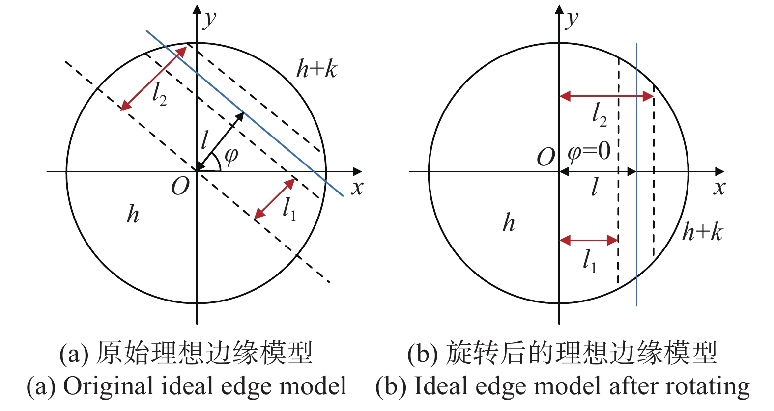
参考文献[18]建立了一种理想的边缘灰度模型,利用Zernike矩的正交性以及旋转不变性对理想阶跃边缘模型进行描述。图1为亚像素边缘检测理想模型,其中直线
$l$ 被单位圆包围的区域代表理想边缘,其两侧的灰度值分别为$h$ 和$h + k$ ,$k$ 代表背景与前景图像之间的灰度差,$l$ 为图像坐标系原点到理想边缘的距离,$\varphi $ 为$l$ 和$x$ 轴的夹角,图1(b)为图1(a)绕原点顺时针旋转$\varphi $ 角度的结果。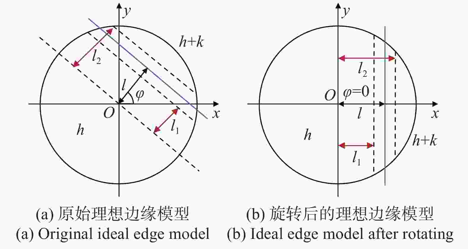
图 1 理想边缘阶跃模型
Figure 1. Ideal step edge model
针对一幅图像,其Zernike矩的形式为:
$${Z_{nm}} = \sum\limits_x {\sum\limits_y {f\left( {x,y} \right){{\mathop V\limits^* }_{nm}}\left( {\rho ,\theta } \right),{x^2} + {y^2} \leqslant 1} } $$ (1) 式中:
${V_{nm}}\left( {\rho ,\theta } \right)$ 表示Zernike多项式;$n$ 与$m$ 表示Zernike矩的阶数;“*”表示共轭变换。Zernike多项式在极坐标下可以表示为:
$$ {V_{nm}}(\rho ,\theta ) = \sum\limits_{s = 0}^{(n - |m|)/2} {\dfrac{{{{( - 1)}^s}(n - s)!{\rho ^{n - 2s}}}}{{s!\left( {\dfrac{{n + |m|}}{2} - s} \right)!\left( {\dfrac{{n - |m|}}{2} - s} \right)!}}} {{\rm e}^{jm\theta }} $$ (2) Zernike矩具有旋转不变性:
$$Z_{nm}' = {Z_{nm}}\exp \left( { - jm\varphi } \right)$$ (3) 根据图1(b)可得,经旋转角度
$\varphi $ 的模型关于$x$ 轴对称,即质心落在$x$ 轴上,满足公式(4)的关系:$$\iint_{{x^2} + {y^2} \leqslant 1} {f'\left( {x,y} \right)y{\rm d}x{\rm d}y} = 0$$ (4) 根据上述等式关系以及Zernike矩的性质,可以列出如下公式:
$$\left\{ \begin{array}{l} Z_{00}' = h\pi + \dfrac{{k\pi }}{2} - k{\arcsin}\left( l \right) - kl\sqrt {1 - {l^{\rm{2}}}} \\ Z_{{\rm{11}}}' = \dfrac{{2k{{\left( {1 - {l^{\rm{2}}}} \right)}^{{3 / 2}}}}}{3},Z_{{\rm{2}}0}' = \dfrac{{2kl{{\left( {1 - {l^{\rm{2}}}} \right)}^{{3 / 2}}}}}{3} \\ Z_{{\rm{31}}}' = k\sqrt {{{\left( {1 - {l^{\rm{2}}}} \right)}^3}} \left( {\dfrac{4}{5}{l^{\rm{2}}} - \dfrac{2}{{15}}} \right) \\ Z_{{\rm{4}}0}' = k\sqrt {{{\left( {1 - {l^{\rm{2}}}} \right)}^3}} \left( {\dfrac{{16}}{{15}}{l^{\rm{3}}} - \dfrac{2}{5}l} \right) \\ \end{array} \right.$$ (5) 理想边缘模型的各个参数可以通过公式(5)求得:
$$\left\{ \begin{array}{l} l = \dfrac{{{Z_{20}}}}{{Z_{11}'}},{l_1} = \sqrt {\dfrac{{5Z_{40}' + 3Z_{20}'}}{{8Z_{20}'}}} \\ {l_2} = \sqrt {\dfrac{{5Z_{31}' + Z_{11}'}}{{6Z_{11}'}}} ,k = \dfrac{{3Z_{11}'}}{{2{{\left( {1 - {l^{\rm{2}}}} \right)}^{3/2}}}} \\ h = \dfrac{{{Z_{00}} - \dfrac{{k\pi }}{2} + k{{\arcsin }}\left( {{l_{\rm{2}}}} \right) + k{l_{\rm{2}}}\sqrt {1 - {l_2}^{\rm{2}}} }}{\pi } \\ \end{array} \right.$$ (6) 因此图像边缘的子像素边缘位置可以表示为:
$$\left[ {\begin{array}{*{20}{c}} {{x_s}}\\ {{y_s}} \end{array}} \right] = \left[ {\begin{array}{*{20}{c}} x\\ y \end{array}} \right] + l\left[ {\begin{array}{*{20}{c}} {\cos \varphi }\\ {\sin \varphi } \end{array}} \right]$$ (7) 式中:
$\left( {{x_s},{y_s}} \right)$ 与$\left( {x,y} \right)$ 分别表示在图像像素坐标系下子像素边缘坐标与Sobel算子提取的边缘坐标。对于一幅图像,Zernike矩是由模板与图像进行卷积计算得到,对于大小为
$N \times N$ 的模板,考虑其放大的作用,边缘像素点可以进一步表示为:$$\left[ {\begin{array}{*{20}{c}} {{x_s}} \\ {{y_s}} \end{array}} \right] = \left[ {\begin{array}{*{20}{c}} x \\ y \end{array}} \right] + \dfrac{N}{2}l\left[ {\begin{array}{*{20}{c}} {\cos \varphi } \\ {\sin \varphi } \end{array}} \right]$$ (8) -
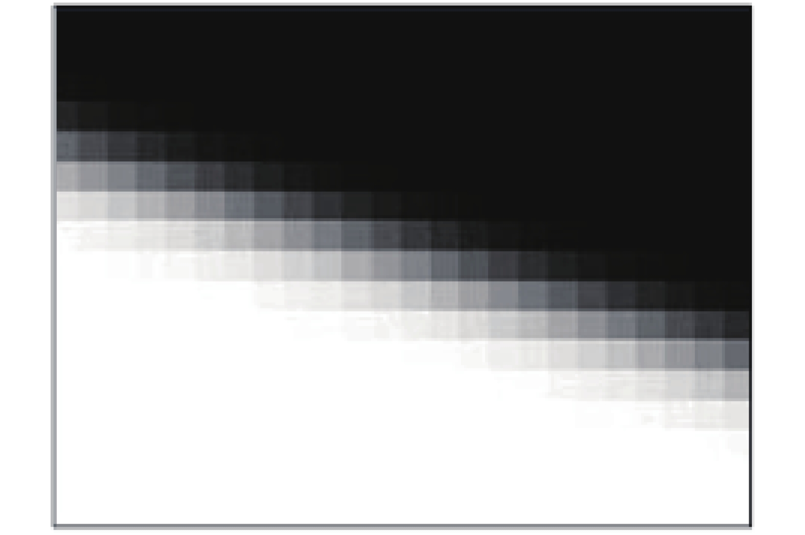
上述基于Zernike矩的亚像素边缘定位方法将实际的边缘简化为三个参数,分别为背景灰度值,边缘灰度阶跃以及边界位置,作为理想化的边缘模型,其并未考虑图像采样过程中的相机透射畸变,传感器噪声以及环境不均匀光照分布等因素,因此不能精确描述图像中边缘的灰度变化。实际图像中的边缘可用连续变化的灰度值表示,且沿着不同的方向灰度值遵循不同变化规律,如图2所示。

图 2 实际图像边缘灰度分布情况
Figure 2. Grayscale distribution of projected ellipse
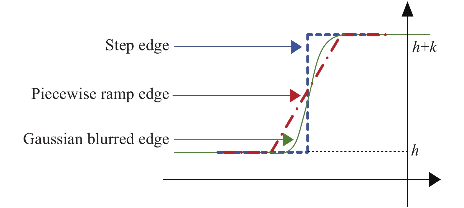
考虑到边缘处的灰度连续变换,引入分段斜坡灰度模型以更精确地描述灰度值变化规律:
$$f\left( x \right) = \left\{ \begin{array}{l} h,\;\;\;\;\;\;\;x < {l_1} \\ h + \dfrac{k}{{{l_2} - {l_1}}}\left( {x - {l_1}} \right),{l_1} \leqslant x < {l_2} \\ h + k,\;\;\;\;\;\;\;{l_2} \leqslant x \\ \end{array} \right.$$ (9) 式中:
$h$ 为背景灰度值;$k$ 为背景与目标灰度差值;${l_1}$ 为边缘的初始位置;${l_2}$ 为边缘的终止位置,图中的边缘位置$l$ 为${l_1}$ ,${l_2}$ 的均值。对于${l_1} < x < {l_2}$ 的边界区域,考虑到灰度变化应为非线性,故对斜坡模型的线性部分使用公式(10)所示的高斯误差函数(erf,error function or Gauss error function)进行优化,得到公式(11)所示的高斯边缘灰度模型:$$erf(x) = \dfrac{2}{{\sqrt \pi }}\int_0^x {{{\rm e}^{ - {t^2}}}} {\rm d}t$$ (10) $$f\left( x \right) = \dfrac{k}{2}\left( {erf\left( {\dfrac{{x - l}}{{\sqrt 2 \sigma }}} \right) + 1} \right) + h$$ (11) 最终可得到描述边缘灰度连续不均匀变换的高斯灰度模型:
$$ {\begin{array}{l} {f_{erf}}\left( {x,{x_i},{y_i}} \right) = \\ \left\{ {\begin{array}{*{20}{c}} h \\ {h + \dfrac{k}{2}\left( {erf\left( {\dfrac{{x - {{\left( {{l_1} + {l_2}} \right)} / 2}}}{{\sqrt 2 \sigma \left( {{x_i},{y_i}} \right)}}} \right) + 1} \right)} \\ {h + k} \end{array}} \right.\begin{array}{*{20}{c}} {}{\begin{array}{*{20}{c}} {x \leqslant {l_1}\left( {{x_i},{y_i}} \right)} \\ {{l_1}\left( {{x_i},{y_i}} \right) < x < {l_2}\left( {{x_i},{y_i}} \right)} \\ {x \geqslant {l_2}\left( {{x_i},{y_i}} \right)} \end{array}} \end{array} \\ \end{array} }$$ (12) 公式(12)考虑了由于光照以及相机采样角度等因素引起的图像边缘灰度不均匀分布,
$\sigma \left( {{x_i},{y_i}} \right)$ 为坐标$\left( {{x_i},{y_i}} \right)$ 为中心的邻域内像素灰度标准差,基于参数估计的方法构建了精确的边缘灰度模型,图3为边缘模型在二维坐标下的表示。
图 3 边缘灰度分布模型二维表示
Figure 3. Two-dimensional representation of edge gray distribution model
将上述边缘模型代入Zernike矩中即可得到考虑边缘模糊的改进Zernike矩,如下式:
$$ {\left\{ \begin{array}{l} Z_{00}' = h\pi + 2\displaystyle\int_{{l_1}}^{{l_2}} {\sqrt {1 - {x^2}} \left( {h - \dfrac{k}{2} \cdot erf\left( {\dfrac{{\sqrt 2 \left( {1 - x} \right)}}{2}} \right) - \dfrac{k}{2}} \right)} {\rm d}x +\\ k\left( {\dfrac{\pi }{2} - {l_2}\sqrt {1 - {l_2}^2} - \arcsin \left( {{l_2}} \right)} \right) \\ Z_{11}' = \dfrac{1}{2}\displaystyle\int_{{l_1}}^{{l_2}} {\left( {2h + k - k \cdot erf\left( {\dfrac{{\sqrt 2 \left( {1 - x} \right)}}{2}} \right)} \right)2x\sqrt {1 - {x^2}} {\rm d}x} + \\ \dfrac{{2k}}{3}\sqrt {{{\left( {1 - l_2^2} \right)}^3}} \\ Z_{20}' = \dfrac{1}{3}\displaystyle\int_{{l_1}}^{{l_2}} {\sqrt {1 - {x^2}} \left( {4{x^2} - 1} \right)\left( {2h + k - k \cdot erf\left( {\dfrac{{\sqrt 2 \left( {1 - x} \right)}}{2}} \right)} \right){\rm d}x} + \\ \dfrac{{2k{l_2}\sqrt {{{\left( {1 - l_2^2} \right)}^3}} }}{3} \\ Z_{31}' = \dfrac{1}{4}\displaystyle\int_{{l_1}}^{{l_2}} {\left( {2h + k - k \cdot erf\left( {\dfrac{{\sqrt 2 \left( {1 - x} \right)}}{2}} \right)} \right)\left( {\gamma \left( {{l_2}{x^3} - 8x} \right)} \right.} + \\ \left. { 4x\sqrt {{{\left( {1 - {x^2}} \right)}^3}} } \right){\rm d}x + \dfrac{{4k}}{{15}}\left( {\sqrt {1 - l_2^2} } \right)\left( {2 + l_2^2 - 3l_2^4} \right) \end{array} \right.}$$ (13) 则有
$Z_{00}'$ 、$Z_{11}'$ 、$Z_{20}'$ 、$Z_{31}'$ 的值为:$$\left\{ \begin{array}{l} Z_{00}' = h\pi + \Delta k\left[ {\arcsin \left( {{l_1}} \right) - \arcsin \left( {{l_2}} \right) + {l_1}\sqrt {1 - l_1^2} } \right. -\\ \left. { {l_2}\sqrt {1 - l_2^2} } \right] + k\left[ {\dfrac{\pi }{2} - {l_2}\sqrt {1 - {l_2}^2} - \arcsin \left( {{l_2}} \right)} \right] \\ Z_{11}' = \dfrac{{2\Delta k}}{3}\left[ {\sqrt {{{\left( {1 - l_1^2} \right)}^3}} - \sqrt {{{\left( {1 - l_2^2} \right)}^3}} } \right] + \dfrac{{2k}}{3}\sqrt {{{\left( {1 - l_2^2} \right)}^3}} \end{array} \right.$$ $$\left\{ \begin{array}{l} Z_{20}' = \dfrac{{2k{l_2}\sqrt {{{\left( {1 - l_2^2} \right)}^3}} }}{3} -\\ \dfrac{{2\Delta k\left( {l_1^3\sqrt {1 - l_1^2} - l_2^3\sqrt {1 - l_2^2} - {l_1}\sqrt {1 - l_1^2} } \right) + {l_2}\sqrt {1 - l_2^2} }}{3} \\ Z_{31}' = \dfrac{{4\Delta k}}{{15}}\left[ {\sqrt {1 - l_1^2} \left( {2 - 3l_1^4 + l_1^2} \right)} \right]- \\ \dfrac{{2\Delta k}}{3}\left( {\sqrt {{{\left( {1 - l_1^2} \right)}^3}} - \sqrt {{{\left( {1 - l_2^2} \right)}^3}} } \right) - \dfrac{{2k}}{{15}}\sqrt {1 - l_2^2} \left( {6l_2^4 - 7l_2^2 + 1} \right) \end{array} \right.$$ (14) 从而进一步得到新的边缘像素定位表达式:
$${l_m} = \dfrac{{Z_{20}'}}{{Z_{11}'}} = \dfrac{{\left( {1 - \dfrac{{\Delta k}}{k}} \right){l_2}\left( {1 - l_2^2} \right)\sqrt {1 - l_2^2} + \dfrac{{\Delta k}}{k}{l_1}\left( {1 - l_1^2} \right)\sqrt {1 - l_1^2} }}{{\dfrac{{\Delta k}}{k}\sqrt {{{\left( {1 - l_2^2} \right)}^3}} + \left( {1 - \dfrac{{\Delta k}}{k}} \right)\sqrt {{{\left( {1 - l_2^2} \right)}^3}} }}$$ (15) 式中的
$\Delta k$ 为:$$\Delta k = \dfrac{k}{2}\int_{{l_1}}^l {\left( {1 + erf\left( {\dfrac{{x - {{\left( {{l_1} + {l_2}} \right)} / 2}}}{{\sqrt 2 \sigma \left( {{x_i},{y_i}} \right)}}} \right)} \right)} {\rm d}x$$ 文中提出的改进Zernike矩考虑了图像中边界像素灰度分布情况,将边界的区域表示为灰度值的连续变化而非灰度值阶跃的形式,更符合实际的情况,同时结合相机成像系统硬件噪声以及环境对相机成像的干扰等因素,利用高斯误差函数进行边界过渡区域的灰度值估计,精确地描述了边界处像素灰度分布情况,利用此边缘模型计算的Zernike矩可以求解得到准确的边缘像素坐标,为后续圆形特征圆心的高精度定位提供了良好的数据基础。
-
对得到的边缘像素坐标进行椭圆拟合,椭圆方程具有如下形式:
$$A{x^2} + Bxy + C{y^2} + Dx + Ey + F = 0$$ (16) 进一步表示为矩阵形式:
$${W^{\rm T}}X = 0$$ (17) 其中:
$$ W = {\left[ {A,B,C,D,E,F} \right]^{\rm T}},X = {\left[ {{x^2},xy,{y^2},x,y,1} \right]^{\rm T}} $$ 拟合椭圆的最优化问题可表示为:
$$\left\{ \begin{gathered} \min {\left\| {{W^{\rm T}}X} \right\|^2} \\ {\rm s.t.}{\rm{ }}{W^{\rm T}}HW = 1 \\ \end{gathered} \right.$$ (18) 其中:
$$H = \left[ {\begin{array}{*{20}{c}} 0&0&2&0&0&0 \\ 0&{ - 1}&0&0&0&0 \\ 0&0&0&0&0&0 \\ 0&0&0&0&0&0 \\ 0&0&0&0&0&0 \\ 0&0&0&0&0&0 \end{array}} \right]$$ 对于上述的约束目标,引入拉格朗日乘子,利用拉格朗日乘子法进行求解即可求得各项参数得到拟合椭圆。但是由于图像采集时环境的干扰以及设备自身硬件的噪声,经边缘定位的边界点包含目标边缘以及部分噪声,为了剔除这部分数据,文中采取迭代拟合椭圆的方法,对每次迭代得到二次曲线进行残差分析,滤除残差较大的边界点进行二次拟合,重复这些步骤直到所有的保留边界点的残差值全部小于设定的阈值则认定拟合椭圆为投影椭圆。
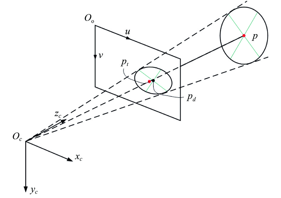
根据针孔成像模型,当空间的圆形特征物理平面不严格垂直于相机的光轴时,空间圆的透视投影成像应为一个椭圆,此变换过程的模型如图4所示。

图 4 空间圆形特征投影成像模型
Figure 4. Spatial circular projection model
图4中,p点为空间圆的中心,其在像平面的投影点为
${p_t}$ ,而投影椭圆的几何中心为${p_d}$ ,在一般情况下${p_t}$ 与${p_d}$ 不重合,且两点的像素坐标分别为:$$ {\left\{ \begin{gathered} {x_{{p_d}}} = \dfrac{{2\left( {{n^2} + {p^2} - \eta _i^2{e^2}} \right)\left( {2mw + 2oq - 2\eta _i^2df} \right)}}{Q} -\\ \dfrac{{\left( {2mn + 2op - 2de\eta _i^2} \right)\left( {2nw + 2pq - 2\eta _i^2ef} \right)}}{Q} \\ {y_{{p_d}}} = \dfrac{{2\left( {{m^2} + {o^2} - \eta _i^2{d^2}} \right)\left( {2mw + 2pq - 2\eta _i^2ef} \right)}}{Q} -\\ \dfrac{{\left( {2mn + 2op - 2de\eta _i^2} \right)\left( {2mw + 2oq - 2\eta _i^2df} \right)}}{Q} \\ {x_{{p_t}}} = \dfrac{{nq - wp}}{{mp - no}} \\ {y_{{p_t}}} = \dfrac{{ow - mq}}{{mp - no}} \\ Q = {\left( {2mn + 2op - 2de\eta _i^2} \right)^2} - 4\left( {{m^2} + {o^2} - \eta _i^2{d^2}} \right)\cdot \\ \left( {{n^2} + {p^2} - \eta _i^2{e^2}} \right) \end{gathered} \right.}$$ (19) 公式(19)中各符号的意义为:
$$\begin{array}{*{20}{l}} \begin{gathered} a = \left( {{r_8}{t_y} - {r_5}{t_z}} \right),b = \left( {{r_2}{t_z} - {r_8}{t_x}} \right),c = \left( {{r_5}{t_x} - {r_2}{t_y}} \right) \\ m = \left( {a - {X_i}d} \right),n = \left( {b - {X_i}e} \right),d = \left( {{r_5}{r_7} - {r_4}{r_8}} \right)\\ \end{gathered}\\ \begin{gathered} e = \left( {{r_1}{r_8} - {r_2}{r_7}} \right),f = \left( {{r_2}{r_4} - {r_1}{r_5}} \right),w = \left( {c - {X_i}f} \right) \\ o = \left( {h + {Y_i}d} \right),h = \left( {{r_7}{t_y} - {r_4}{t_z}} \right),j = \left( {{r_1}{t_z} - {r_7}{t_x}} \right)\\ \end{gathered}\\ {k = \left( {{r_4}{t_x} - {r_1}{t_y}} \right),p = \left( {j + {Y_i}} \right),q = \left( {k + {Y_i}f} \right)} \end{array}$$ 式中:
$({X_i},{Y_i})$ 为空间圆上各点的世界坐标;${\eta _i}$ 为半径;$t$ 为相机外参中的平移分量;${r_i}$ 为旋转矩阵中的元素。又已知这两点并不重合,以两点之间的偏移量作为圆形特征投影的畸变误差:$$\Delta = \sqrt {{{({x_{{p_t}}} - {x_{{p_d}}})}^2} + {{\left( {{y_{{p_t}}} - {y_{{p_d}}}} \right)}^2}} $$ (20) 分析上式所述畸变误差,根据参考文献[7]魏振忠等人的仿真分析结果,此畸变项受空间圆心和像平面距离以及空间圆平面和像平面的夹角影响,误差会随着物象距离的增大而减小,随着物象夹角的减小而减小,误差最小可达
$5.2$ μm,而在文中的相机标定过程中,物象距离较远且圆特征与相机成像平面的夹角较小,因此获得高精度逼近投影椭圆几何中心的拟合圆心坐标对于获得更好的标定效果很有必要。对得到和拟合圆心进一步处理逼近真实的投影椭圆几何中心。处理边缘坐标,获取距离最远的两个点,其连线认定为椭圆长轴,中点为椭圆圆心,比较中点与拟合圆心的距离,此距离小于设定阈值将两点的中点作为投影圆心坐标,否则计算两点连线与投影椭圆的交点
$({u_1},{v_1})$ 和$\left( {{u_2},{v_2}} \right)$ ,根据射影变换的简比不变与直线不变原则,得到高精度的圆心投影点坐标$\left( {{u_o},{v_o}} \right)$ 为:$$\left\{ \begin{gathered} \dfrac{{{u_o} - {u_1}}}{{{u_2} - {u_1}}} = \dfrac{R}{{2R}} \\ \dfrac{{{v_o} - {v_1}}}{{{v_2} - {v_1}}} = \dfrac{R}{{2R}} \\ \end{gathered} \right. \Rightarrow \left\{ \begin{gathered} {u_o} = \dfrac{{{u_1} + {u_2}}}{2} \\ {v_o} = \dfrac{{{v_1} + {v_2}}}{2} \\ \end{gathered} \right.$$ (21) 式中:R的为空间圆形特征的半径。
通过以上方法可以对得到的拟合椭圆圆心进行补偿误差,得到高精度逼近真实投影点的坐标值,算法流程图如图5所示。
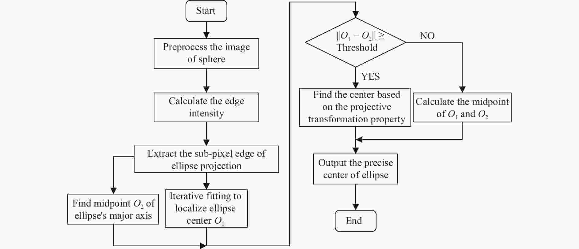
图 5 投影椭圆拟合算法流程图
Figure 5. Projection ellipse fitting algorithm
-
基于亚像素的灰度图像边缘定位方法有:灰度矩法,拟合法,Zernike矩法等,为了对文中所提出的改进Zernike矩算法进行定位精度的评估,将其分别与上述三种方法在仿真实验中进行比较,并对改进算法的鲁棒性和定位精度进行分析。
为了对上述几种亚像素边缘定位算法的定位精度和鲁棒性进行比较,文中基于绘图工具绘制了大小为1 680
$ \times $ 1 680 pixel的黑底白圆模拟图像,如图6所示,圆心坐标为(256,256),半径$r = {\rm{5}}0$ pixel,为了模拟实际情况,将方差为0,0.002,0.004的高斯白噪声加入到模拟图像中,通过分析上述三种传统方法以及文中算法对模拟图像边缘提取的误差分布和圆心定位偏差大小来验证所提方法的有效性和鲁棒性。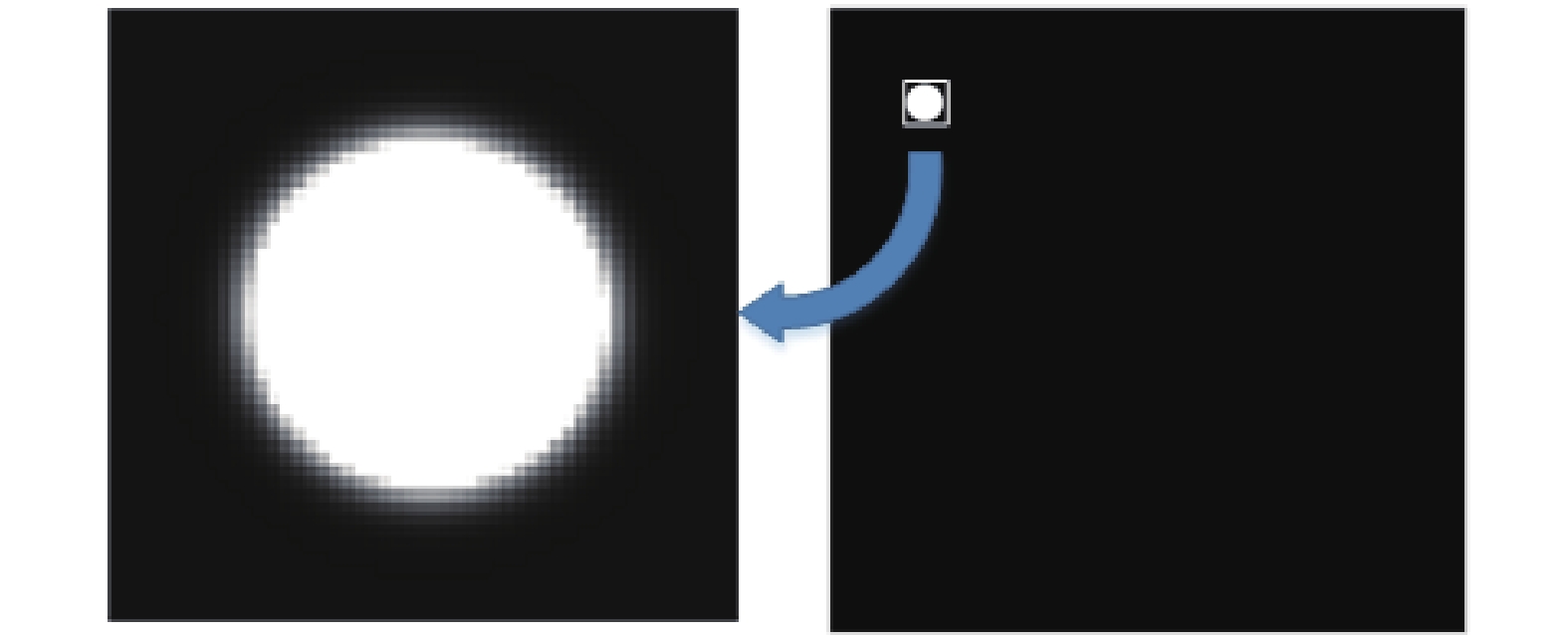
图 6 仿真模拟图像
Figure 6. Simulative image
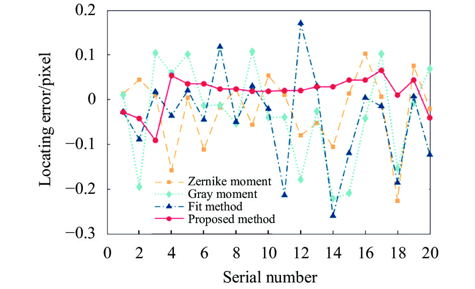
图7为模拟图像加入了方差为0.002的高斯白噪声时,用四种方法对圆形特征边缘定位与边缘真值的误差曲线对比图。从图中可以看出,对于相同噪声水平的模拟图像,文中所提算法的定位误差明显小于其他三种传统算法,误差分布更接近0,由此可见文中算法对图像噪声的敏感度较低,有较好的抗干扰能力。
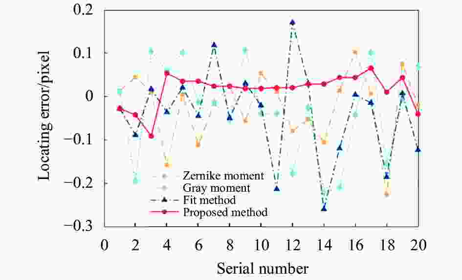
图 7
${\sigma ^{\rm{2}}}$ =0.002的误差分布Figure 7. Error distribution of
${\sigma ^{\rm{2}}}{\rm{ = 0}}{\rm{.002}}$ 对每次实验得到的边缘点坐标进行随机抽样,获取50个样本数据并计算边缘点与圆心的距离,与半径真值作差并计算误差绝对值,然后计算误差绝对值的均值与方差,得到表1的数据。可以看出,在没有噪声干扰的情况下,四种拟合方法都有较高的定位精度,但是随着加入的噪声增强,四种算法的定位误差均逐渐增大,但是文中算法计算的边缘坐标误差均值最小,且相对于其他算法的抗干扰性更强,在不同的噪声等级下误差均值与方差都是最小的,因此可以看出文中算法的抗噪性能最好,精度最高。
表 1 模拟图像边缘定位精度对比表
Table 1. Edge location accuracy of simulative image
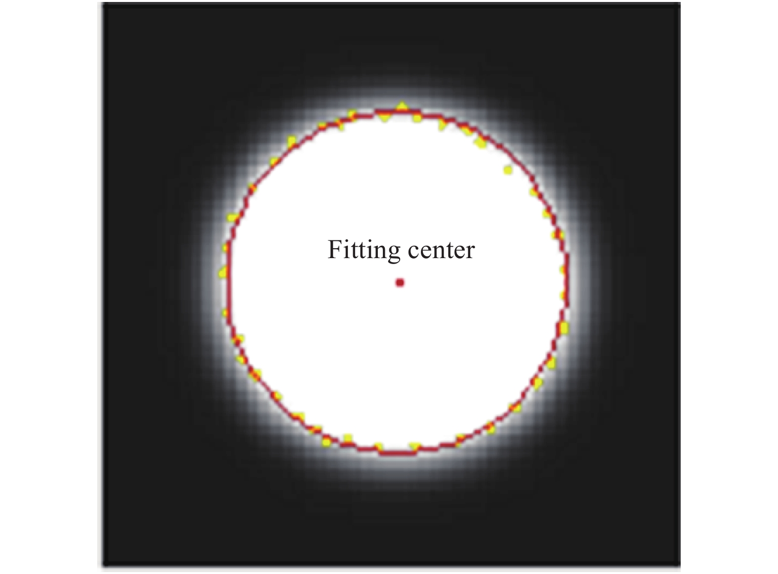
Locate method Type of noise No noise White noise(${\sigma ^{\rm{2}}}$=0.002) White noise(${\sigma ^{\rm{2}}}$=0.004) Mean error/pixel Variance/pixel2 Mean error/pixel Variance/pixel2 Mean error/pixel Variance/pixel2 Gray moment 0.0666 0.0172 0.0807 0.0232 0.1218 0.1979 Fit method 0.0727 0.0363 0.0821 0.0443 0.3277 0.1843 Zernike moment 0.0501 0.0198 0.0867 0.0307 0.1064 0.2512 Proposed method 0.0469 0.0130 0.0564 0.0312 0.0687 0.0866 得到了模拟图像的边缘像素坐标之后,利用这些边界点进行迭代拟合获取其圆心坐标。基于文中算法对模拟图像处理,得到的边缘点以及拟合椭圆如图8所示。

图 8 基于改进Zernike矩的边缘及圆心定位
Figure 8. Edge and center localization based on improved Zernike moments
计算每次提取得到的拟合圆心与模拟图像圆心真值的距离偏差值,得到表2中的数据。从表2中数据可以看出,在相同噪声水平下,文中提出的算法对于圆形特征的圆心定位精度是最高的,相较Zernike矩,文中算法由于使用了更精确的高斯边缘模型计算得到的改进Zernike矩,精度较之提升了约25%。与此同时,由于文中在拟合计算投影椭圆曲线时采用了迭代拟合,滤除野点的方法,可以降低噪声对定位的干扰,进一步增强算法的抗干扰能力。
表 2 模拟图像圆心定位精度对比表
Table 2. Center location accuracy of simulative image
Locate method Type of noise No noise White noise(${\sigma ^{\rm{2}}}$=0.002) White noise(${\sigma ^{\rm{2}}}$=0.004) Fitting center Error/pixel Fitting center Error/pixel Fitting center Error/pixel Gray moment (256.034,256.025) 0.0422 (256.024,255.951) 0.0546 (256.031,256.056) 0.0640 Fit method (255.994,256.041) 0.0417 (255.967,256.165) 0.1683 (256.226,256.186) 0.2926 Zernike moment (255.964,256.022) 0.0414 (255.959,256.014) 0.0430 (255.95,256.012) 0.0511 Proposed method (256.027,255.991) 0.0289 (256.025,255.979) 0.0326 (256.031,255.986) 0.0339 相机标定的精度会受到圆形标志圆心提取误差,标定板精度,镜头畸变等因素的影响,通过仿真实验可以看出文中提出的算法对于圆形特征中心有较高的定位精度,且具有一定的噪声抑制能力,可以在标定过程中得到精确的圆形标志点图像坐标为双目视觉系统的标定提供良好的数据基础。
-
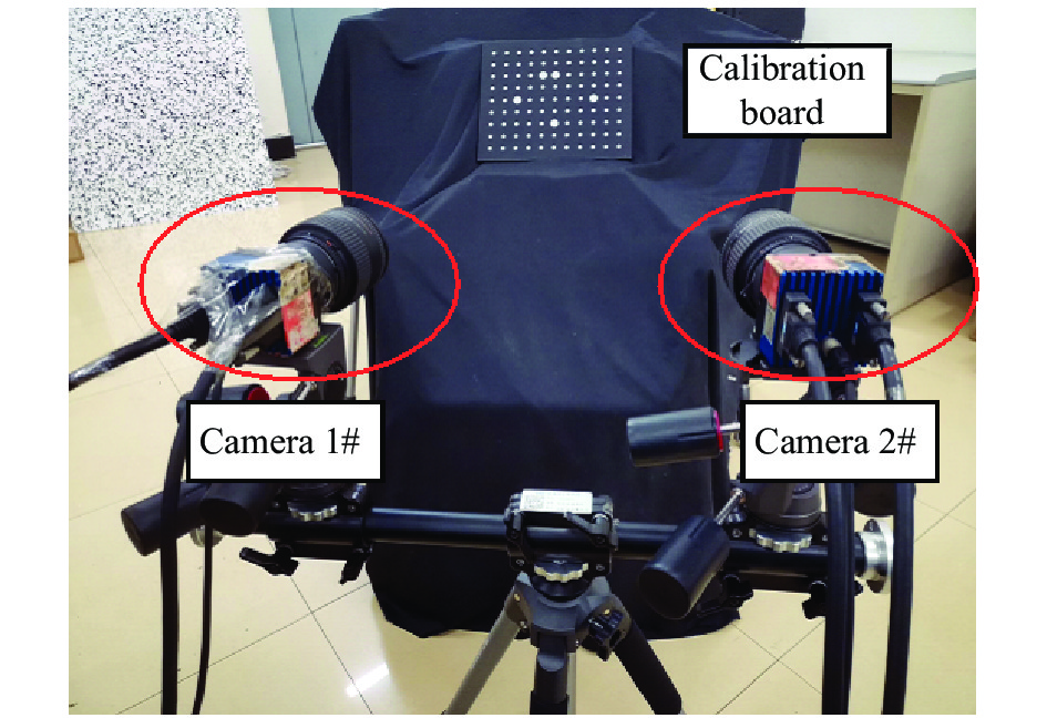
通过仿真实验验证了文中算法能够对圆心特征投影中心进行高精度的提取,为了进一步验证算法对相机标定效果的提升,设计实际标定实验计算相机参数并通过标准杆来对相机标定精度进行检验。构建双目立体视觉系统架构如图9所示,采用两台由Mikrotron生产的MC3010相机,相机图像分辨率为1680×1720 pixel,像元尺寸为
${\rm d}u \times {\rm d}v =$ 7.4 μm×7.4 μm,相机镜头型号均为AF Zoom-Nikkor 24-85 mm/1:2.8-4D,用其拍摄99圆形标定板进行标定完成文中标定方法的验证。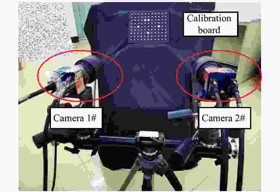
图 9 立体相机系统图像采集设备
Figure 9. Acquisition equipment of stereo camera system image
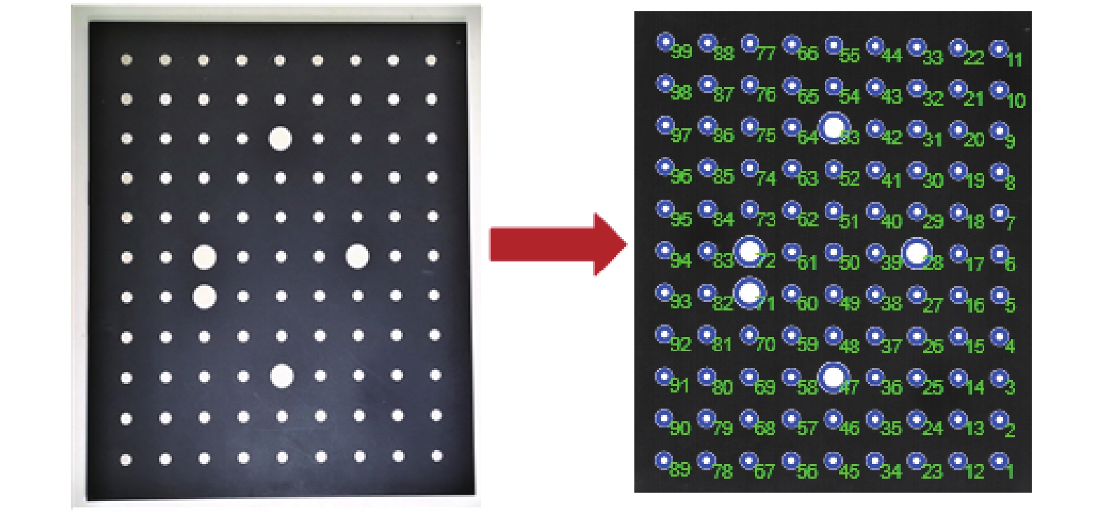
设置圆形标定板位于双目中线方向约1200 mm的位置,通过图9中所示的双目立体成像系统对其进行图像采集,并对标定板上的99个圆形标志点进行圆心提取与编号,如图10所示。

图 10 圆形标志点提取与编码
Figure 10. Extraction and coding of circular mark points
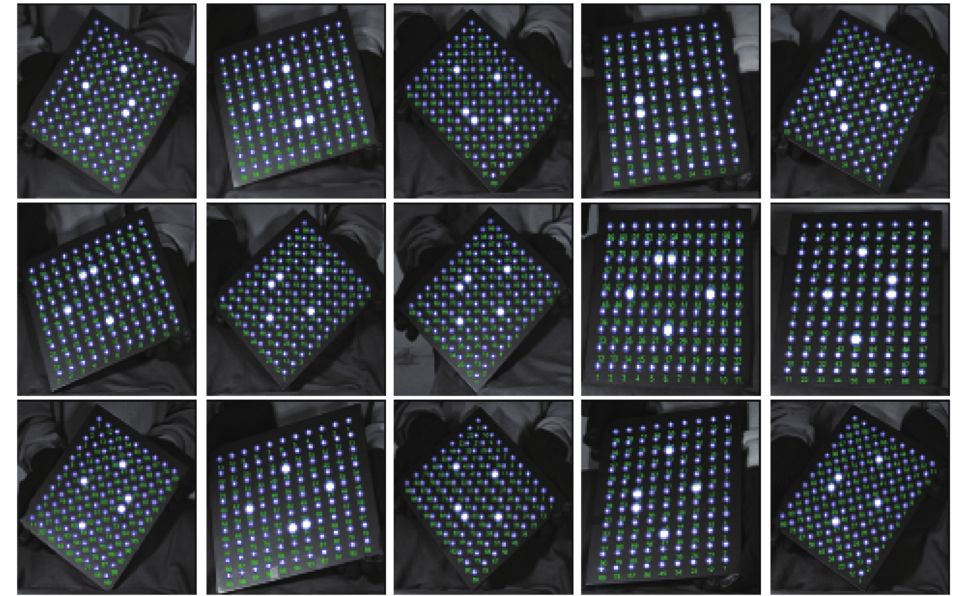
调整平面标定板的姿态,空间位置,使其占据视觉系统的视场大部分区域,通过文中算法对标定板的圆形特征圆心进行高精度提取,并将得到的圆心依次进行编码,图11为部分处于不同位姿状态的标定板图像及编码情况。

图 11 标靶图像采集与圆心提取效果
Figure 11. Target image acquisition and center extraction
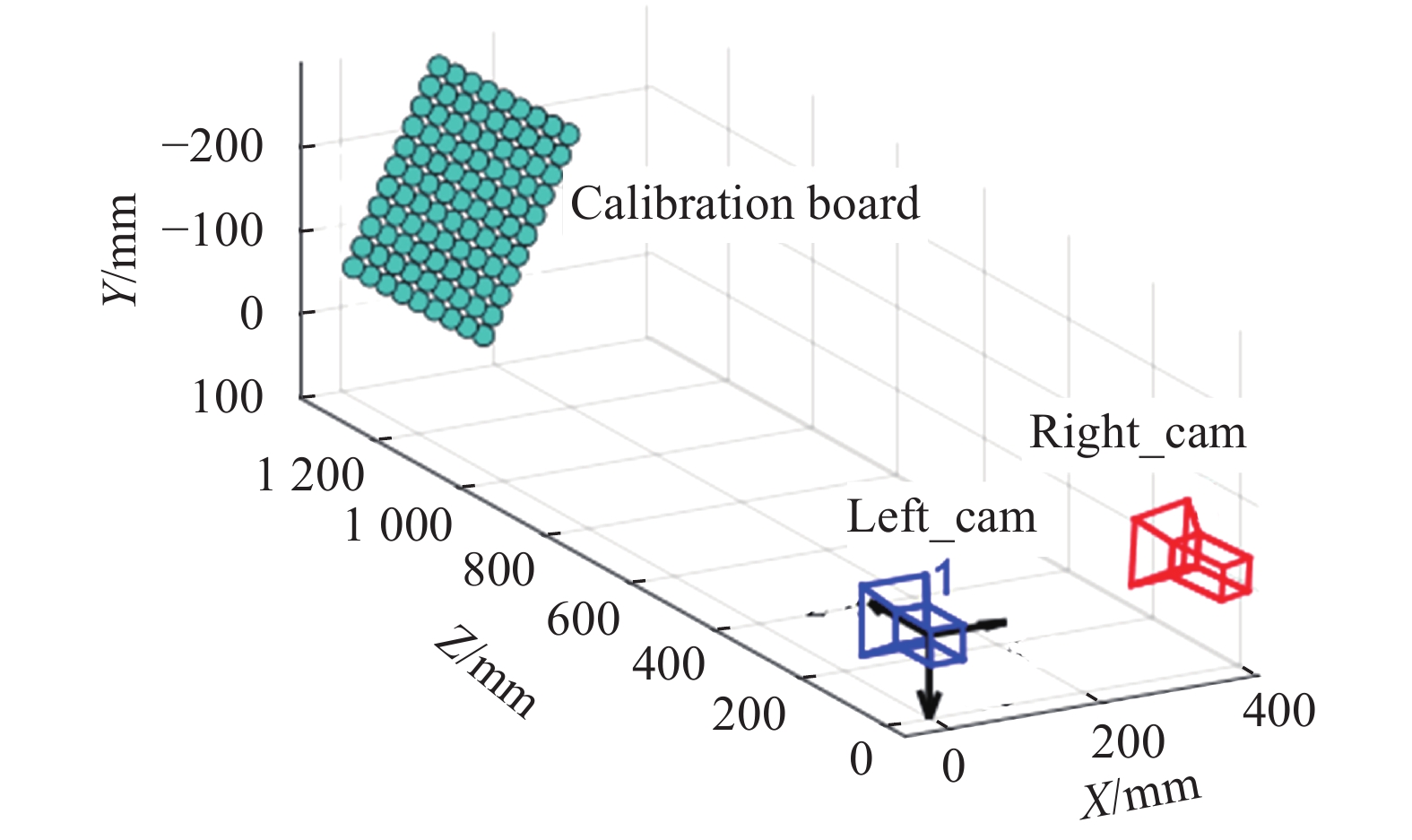
此次标定实验中双目立体视觉系统左右相机分别采集了25张标定板图像,对所有图像中的圆形标志点利用文中方法进行圆心的高精度定位求解图像坐标,并依据图像和标定板的对应关系以及标定板各个圆形特征的几何关系计算双目相机系统的相机参数。表3为通过文中算法解算出的相机参数以及双目之间的位姿关系。图12为基于标定结果重构的标定板特征点空间三维分布效果图以及双目相机和标定板的空间位姿关系。
表 3 相机内参及双目位姿关系
Table 3. Camera internal parameters and binocular posture relationship
Left camera’s intrinsics Right camera’s intrinsics Extrinsics ${f_x} = {\rm{3051}}{\rm{.903\;4}}$
${f_y} = {\rm{3051}}{\rm{.349\;0}}$
${u_0} = {\rm{836}}{\rm{.169\;0}}$
${v_0} = {\rm{910}}{\rm{.385\;3}}$
${k_1} = - {\rm{0}}{\rm{.176\;9}}$
${k_2} = {\rm{0}}{\rm{.189\;4}}$
$s = 0$${f_x} = {\rm{3\;085}}{\rm{.834\;1}}$
${f_y} = {\rm{3\;087}}{\rm{.418\;6}}$
${u_0} = {\rm{812}}{\rm{.227\;4}}$
${v_0} = {\rm{859}}{\rm{.930\;4}}$
${k_1} = - {\rm{0}}{\rm{.182\;0}}$
${k_2} = {\rm{0}}{\rm{.375\;9}}$
$s = 0$$\begin{gathered} R = \left[ {\begin{array}{*{20}{c}} {0.965\;3}&{0.006\;2}&{ - 0.261\;1} \\ { - 0.040\;2}&{0.991\;3}&{ - 0.125\;1} \\ {0.258\;1}&{0.131\;2}&{0.957\;2} \end{array}} \right] \\ T = \left[ {\begin{array}{*{20}{c}} {{\rm{ - 363}}{\rm{.001\;5}}}&{{\rm{14}}{\rm{.625\;0}}}&{{\rm{86}}{\rm{.082\;6}}} \end{array}} \right] \\ \end{gathered} $ 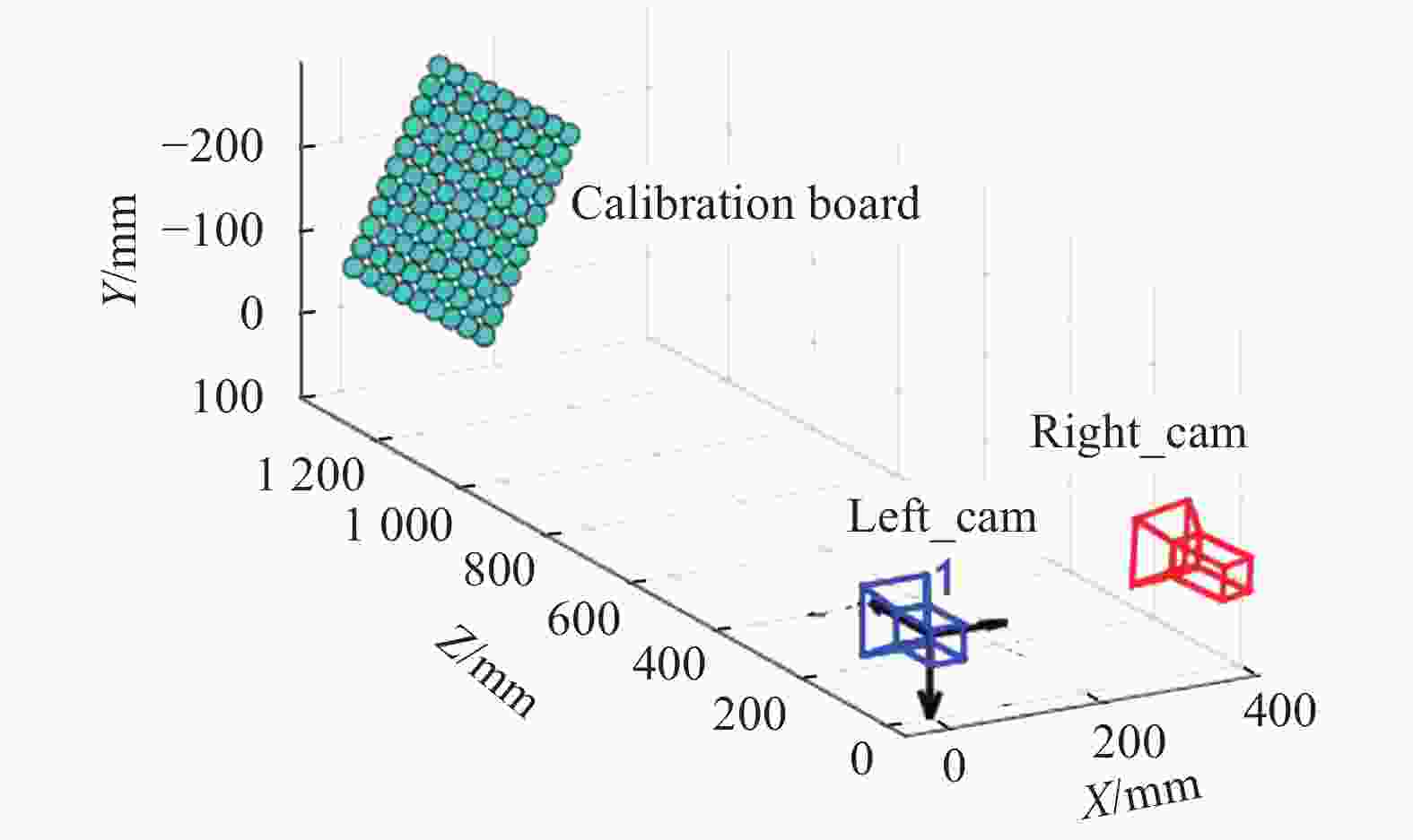
图 12 立体视觉系统标定结果
Figure 12. Stereo vision system calibration results
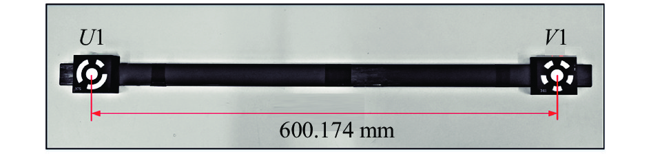
然后利用如图13所示的标准杆对双目视觉系统的标定结果进行精度验证,将标准杆放置于立体视觉系统的视场范围内并采集图像,分别利用灰度矩,拟合法,Zernike矩以及Hough变换等传统做法与文中算法得到的相机参数对标准杆采样图像进行重构,获得标准杆的两端标志点的坐标,考虑到物体在世界坐标系下的实际坐标不易获得,因此设计实验使用文中算法标定获取的相机参数对标准杆件进行长度测量,然后与标准杆长度真值比较并计算测量误差,各个方案多次测量得到的平均结果如表4所示。

图 13 实测标定杆
Figure 13. Calibration rod
表 4 标定杆测量精度对比表
Table 4. Calibration rod measurement accuracy
Method Fitting center A Fitting center B Length/mm Error/mm Gray moment (317.588,−237.967,1250.752) (−223.332,9.369,1172.507) 599.9098 0.2642 Fit method (317.607,−237.573,1250.357) (−223.792,9.302,1173.957) 599.9142 0.2598 Zernike moment (317.624,−237.219,1251.199) (−223.726,9.496,1173.864) 599.9240 0.2500 Hough transform (317.701,−237.186,1250.309) (−223.912,9.357,1174.357) 599.9147 0.2593 Proposed method (317.486,−238.568,1249.487) (−223.325,9.329,1171.598) 599.9968 0.1772 表4中的数据显示,基于文中算法优化的标定方法得到的双目视觉系统参数将测量误差值控制在0.2 mm以内,明显小于其他四种传统做法的测量结果,测量精度提升约30%,可以看出文中算法在提升标定精度上具有一定的优势。这是因为传统的标定做法中,忽略了圆形特征投影时存在的偏心误差以及圆形特征投影的边缘模糊问题,在计算标定板圆形特征的圆心时引入了较大的误差;而文中算法通过建立了高斯边缘模型精确描述了圆形特征的边缘并且补偿了偏心误差,因此能够实现更高精度的相机标定。
文中提出的算法考虑了由于干扰引起的圆形特征投影边缘模糊以及投影偏心问题,提出了更适合描述此类边缘灰度分布的边缘模型并基于此模型计算图像的Zernike矩实现亚像素定位,最终利用高精度的定位坐标数据进行拟合并补偿圆心误差,以此圆心坐标进行相机标定得到的相机参数相对传统方法有更高精度,但是此算法也因为加入了更多的计算,在标定过程中相比传统做法存在运行时间长的问题,这也将是未来工作需要着力去改进的地方。
-
文中考虑了在相机标定过程中由于相机本身的传感器噪声以及环境光照分布不均等因素引起的圆形特征投影边缘模糊现象,引入高斯误差函数建立了高斯边缘灰度分布模型,并基于此模型计算图像的Zernike矩来实现边缘的亚像素定位,然后利用高精度的亚像素坐标迭代拟合得到投影椭圆的拟合圆心坐标,并通过分析投影几何圆心和真实投影中心的偏离关系,对拟合圆心进行补偿误差,最终基于此圆心坐标对立体视觉系统进行标定得到相机参数。通过仿真实验和实测实验可以验证该算法的有效性和准确性,文中提出的算法在边缘像素坐标提取和圆心拟合上均优于四种传统算法,对于标准杆的三维重建测量精度也比传统算法提升了30%,能够满足高精度的三维测量任务,具有实际的工程应用价值。
下一步工作将针对文中算法计算量大、标定时间久的问题进行改进,可以通过GPU进行并行运算,基于异构加速提高算法的运行效率。
High-precision camera calibration method considering projected circular edge blur and eccentricity error
-
摘要: 针对立体视觉系统采用圆形特征点标定时存在的空间圆形投影边缘模糊和偏心现象问题,利用改进Zernike矩和偏心误差修正进行圆心的高精度定位,以此提高相机参数的标定精度。首先考虑了由于立体视觉成像系统的标定场景光照强度不均匀引起的圆形特征投影图像边缘模糊的问题,引入高斯误差函数对边缘过渡段的灰度分布进行描述,建立了高斯边缘模型,并基于该模型计算投影图像的Zernike矩,然后利用改进Zernike矩实现高精度的圆形特征投影边缘像素坐标定位。此外,分析了影响圆形特征中心投影点和拟合圆心间偏差大小的因素,基于该分析对迭代拟合圆心进行偏差补偿使之逼近真实的圆心投影,最后通过所提算法对99圆形标志点进行圆心坐标提取并用于相机参数的标定。仿真实验表明,文中算法对投影图像边缘定位的精度以及圆心拟合的精度均高于传统的算法;实测实验中,基于圆心高精度坐标得到的相机标定参数对标准杆进行三维重建,长度测量精度比传统算法提高了30%。
-
关键词:
- 立体视觉 /
- 改进Zernike矩 /
- 偏心误差修正 /
- 相机标定
Abstract: In order to improve the calibration accuracy of camera parameters, the improved Zernike moment and eccentricity error correction were used to locate the center of the circle with high accuracy for the problem of blurred edges and eccentricity of spatial circular projection when calibrating with circular feature points in stereo vision system. The problem of blurred edges of circular feature projection image caused by uneven illumination intensity at the calibration site of stereo vision imaging system was firstly considered, and the Gaussian error function was introduced to describe the grayscale distribution of the edge transition section. The Gaussian edge model was established, and Zernike moments of the projection image were calculated based on this model, and then the improved Zernike moments were used to achieve high-precision circular feature projection edge pixel coordinate positioning. In addition, the factors that affecting the deviation between the projection point of the circular feature and the fitted circle center were analyzed, and the deviation compensation of the iterative fitted circle center was made based on this analysis to make it close to the real circle center projection, and lastly the circle centers of 99 circular marker points were extracted and used for the calibration of the camera parameters by the proposed algorithm. The simulation experiments show that the accuracy of the algorithm for edge positioning of the projected image and the accuracy of the circle center fitting are higher than those of the traditional algorithm; In the practical measurement experiments, it turns out that the length measurement accuracy of standard rod based on the proposed method is improved by 30% compared with traditional methods. -
图 3 边缘灰度分布模型二维表示
Figure 3. Two-dimensional representation of edge gray distribution model
图 7
${\sigma ^{\rm{2}}}$ =0.002的误差分布Figure 7. Error distribution of
${\sigma ^{\rm{2}}}{\rm{ = 0}}{\rm{.002}}$
图 8 基于改进Zernike矩的边缘及圆心定位
Figure 8. Edge and center localization based on improved Zernike moments
表 1 模拟图像边缘定位精度对比表
Table 1. Edge location accuracy of simulative image
Locate method Type of noise No noise White noise( ${\sigma ^{\rm{2}}}$ =0.002)White noise( ${\sigma ^{\rm{2}}}$ =0.004)Mean error/pixel Variance/pixel2 Mean error/pixel Variance/pixel2 Mean error/pixel Variance/pixel2 Gray moment 0.0666 0.0172 0.0807 0.0232 0.1218 0.1979 Fit method 0.0727 0.0363 0.0821 0.0443 0.3277 0.1843 Zernike moment 0.0501 0.0198 0.0867 0.0307 0.1064 0.2512 Proposed method 0.0469 0.0130 0.0564 0.0312 0.0687 0.0866  下载: 导出CSV
表 2 模拟图像圆心定位精度对比表
Table 2. Center location accuracy of simulative image
Locate method Type of noise No noise White noise( ${\sigma ^{\rm{2}}}$ =0.002)White noise( ${\sigma ^{\rm{2}}}$ =0.004)Fitting center Error/pixel Fitting center Error/pixel Fitting center Error/pixel Gray moment (256.034,256.025) 0.0422 (256.024,255.951) 0.0546 (256.031,256.056) 0.0640 Fit method (255.994,256.041) 0.0417 (255.967,256.165) 0.1683 (256.226,256.186) 0.2926 Zernike moment (255.964,256.022) 0.0414 (255.959,256.014) 0.0430 (255.95,256.012) 0.0511 Proposed method (256.027,255.991) 0.0289 (256.025,255.979) 0.0326 (256.031,255.986) 0.0339
下载: 导出CSV
表 3 相机内参及双目位姿关系
Table 3. Camera internal parameters and binocular posture relationship
Left camera’s intrinsics Right camera’s intrinsics Extrinsics ${f_x} = {\rm{3051}}{\rm{.903\;4}}$ ${f_y} = {\rm{3051}}{\rm{.349\;0}}$ ${u_0} = {\rm{836}}{\rm{.169\;0}}$ ${v_0} = {\rm{910}}{\rm{.385\;3}}$ ${k_1} = - {\rm{0}}{\rm{.176\;9}}$ ${k_2} = {\rm{0}}{\rm{.189\;4}}$ $s = 0$ ${f_x} = {\rm{3\;085}}{\rm{.834\;1}}$ ${f_y} = {\rm{3\;087}}{\rm{.418\;6}}$ ${u_0} = {\rm{812}}{\rm{.227\;4}}$ ${v_0} = {\rm{859}}{\rm{.930\;4}}$ ${k_1} = - {\rm{0}}{\rm{.182\;0}}$ ${k_2} = {\rm{0}}{\rm{.375\;9}}$ $s = 0$ $\begin{gathered} R = \left[ {\begin{array}{*{20}{c}} {0.965\;3}&{0.006\;2}&{ - 0.261\;1} \\ { - 0.040\;2}&{0.991\;3}&{ - 0.125\;1} \\ {0.258\;1}&{0.131\;2}&{0.957\;2} \end{array}} \right] \\ T = \left[ {\begin{array}{*{20}{c}} {{\rm{ - 363}}{\rm{.001\;5}}}&{{\rm{14}}{\rm{.625\;0}}}&{{\rm{86}}{\rm{.082\;6}}} \end{array}} \right] \\ \end{gathered} $
下载: 导出CSV
表 4 标定杆测量精度对比表
Table 4. Calibration rod measurement accuracy
Method Fitting center A Fitting center B Length/mm Error/mm Gray moment (317.588,−237.967,1250.752) (−223.332,9.369,1172.507) 599.9098 0.2642 Fit method (317.607,−237.573,1250.357) (−223.792,9.302,1173.957) 599.9142 0.2598 Zernike moment (317.624,−237.219,1251.199) (−223.726,9.496,1173.864) 599.9240 0.2500 Hough transform (317.701,−237.186,1250.309) (−223.912,9.357,1174.357) 599.9147 0.2593 Proposed method (317.486,−238.568,1249.487) (−223.325,9.329,1171.598) 599.9968 0.1772
下载: 导出CSV
-
[1] 张广军, 视觉测量[M]. 北京: 科学出版社, 2008: 134-173. Zhang Guangjun. Vision Measurement[M]. Beijing: Science Press, 2008: 134-173. (in Chinese) [2] Zhang Guiyang, Huo Ju, Yang Ming, et al. Bidirectional closed cloud control for stereo vision measurement based on multi-source data [J]. Acta Optica Sinica, 2020, 40(19): 1915002. (in Chinese) doi: 10.3788/AOS202040.1915002 [3] Liu Wei, Li Xiao, Ma Xin, et al. Camera calibration method for close range large field of view camera based on compound target [J]. Infrared and Laser Engineering, 2016, 45(7): 0717005. (in Chinese) doi: 10.3788/IRLA201645.0717005 [4] Zhang Z. A flexible new technique for camera calibration [J]. IEEE Transactions on Pattern Analysis and Machine Intelligence, 2000, 22(11): 1330-1334. doi: 10.1109/34.888718 [5] Bi Chao, Hao Xue, Liu Mengchen, et al. Study on calibration method of rotary axis based on vision measurement [J]. Infrared and Laser Engineering, 2020, 49(4): 0413004. (in Chinese) doi: 10.3788/IRLA202049.0413004 [6] Zou Yuanyuan, Li Pengfei, Zuo Kezhu. Field calibration method for three-line structured light vision sensor [J]. Infrared and Laser Engineering, 2018, 47(6): 0617002. (in Chinese) doi: 10.3788/IRLA201847.0617002 [7] Wei Zhenzhong, Zhang Guangjun. A distortion error model of the perspective projection of ellipse center and its simulation [J]. Chinese Journal of Scientific Instrument, 2003, 24(2): 160-164. (in Chinese) doi: 10.3321/j.issn:0254-3087.2003.02.014 [8] Xia R X, Lu R S, Liu N, et al. A method of automatic extracting feature point coordinates based on circle array target [J]. China Mechanical Engineering, 2010, 21(16): 1906-1910. (in Chinese) [9] Xie Z X, Wang X M. Research on extraction algorithm of projected circular centers of marked points on the planar calibration targets [J]. Optics and Precision Engineering, 2019, 27(2): 440-449. (in Chinese) doi: 10.3788/OPE.20192702.0440 [10] Lu X D, Xue J P, Zhang Q C. High camera calibration method based on true coordinate computation of circle center [J]. Chinese Journal of Lasers, 2020, 47(3): 0304008. (in Chinese) doi: 10.3788/CJL202047.0304008 [11] Chen Q, Wu H, Wada T. Camera calibration with two arbitrary coplanar circles[C]//Proc European Conf Computer Vision, 2004: 521-532. [12] Li Z L, Liu M, Sun Y. Research on calculation method for the projection of circular target center in photogrammetry [J]. Chinese Journal of Scientific Instrument, 2011, 32(10): 2235-2241. (in Chinese) [13] Ye J, Fu G, Poudel U P. High-accuracy edge detection with blurred edge model [J]. Image and Vision Computing, 2005, 23(5): 453-467. doi: 10.1016/j.imavis.2004.07.007 [14] Liu M P, Zhu W B, Ye S L. Sub-pixel edge detection based on improved Zernike moment in the small modulus gear image [J]. Chinese Journal of Scientific Instrument, 2018, 39(8): 259-267. (in Chinese) [15] Huang X X, Lv Y, Liu L S. Research on sub-pixel location algorithm of infrared image edge [J]. Laser Journal, 2020, 41(12): 57-60. (in Chinese) doi: 10.14016/j.cnki.jgzz.2020.12.057 [16] Chen K, Feng H J, Xu Z H, et al. Sub-pixel location algorithm for planetary center measurement [J]. Optics and Precision Engineering, 2013, 21(7): 1881-1890. (in Chinese) doi: 10.3788/OPE.20132107.1881 [17] Wang N, Duan Z Y, Zhao W H, et al. Algorithm of edge detection based on Bertrand surface model [J]. Acta Photonica Sinica, 2017, 46(10): 1012003. (in Chinese) doi: 10.3788/gzxb20174610.1012003 [18] Ghosal S, Mehrotra R. Orthogonal moment operators for subpixel edge detection [J]. Pattern Recognition, 1993, 26(2): 295-306. doi: 10.1016/0031-3203(93)90038-X -

 点击查看大图
计量
- 文章访问数: 439
- HTML全文浏览量: 119
- PDF下载量: 88
- 被引次数: 0


