


 下载:
下载:

-
散射环境中偏振传输作为能够促进偏振技术发展的重要问题,近年来备受各国研究机构重视。散射偏振特性是丰富且敏感的,研究散射偏振传输规律利于提高信号质量[1-2]、增加传输距离[3]、乃至反演环境属性[4]。
目前,散射偏振传输规律计算主要采用离散坐标法[5]、球谐函数法[6]、倍加累加法[7]、蒙特卡洛法[8]、二流近似法[9]等。其中,蒙特卡洛法由于不存在有限离散引起的计算误差,通常作为验证其他方法计算精度的标准。John等[10-11]采用偏振子午面蒙特卡洛法计算了偏振光在聚苯乙烯悬浊液中的前向传输特性,验证实验表明:测试与计算结果趋势一致,但测试与计算结果存在一定出入。他们[12]分析造成测试和计算结果两者差异的原因可能是计算过程中设置接收截面无限大所致。Slade等[13]采用偏振子午面蒙特卡洛法计算了线偏振光在聚苯乙烯悬浊液和粉尘悬浊液的前向传输情况,验证实验表明:对于聚苯乙烯悬浊液,测试和计算结果趋势基本吻合,但测试与计算结果仍存在一定出入;对于粉尘悬浊液,测试与计算结果趋势差异显著。John与Slade的研究存在共性问题,而聚苯乙烯悬浊液是一种参量可控的实验环境,实验测试本身引入误差较小,因此,测试与计算结果之间的出入主要由计算方式引起,为提高计算与测试之间的匹配程度,尚需对计算方法改进优化。Ghosh等[14] 测试了偏振度与接收角度的关系,实验选用粒径分别为0.11 μm和1.08 μm的单分散聚苯乙烯悬浊液,测试结果表明:随着接收角度的增加,两组环境的偏振度都逐渐下降。Ghosh的研究对算法改进有所启示,目前采用偏振子午面蒙特卡洛法计算时通常未对接收范围进行限定,而实际测试过程中难以采集全部前向散射光,限定接收范围可能是提高算法精度的有效途径之一。
文中为解决偏振子午面蒙特卡洛法的计算与测试结果存在出入的问题,对偏振子午面蒙特卡洛法优化改进。改进算法限定了前向散射光的接收范围,限定的接收范围与实际接收范围一致。通过验证实验,判定改进算法比原算法是否具有更高的计算精度。通过计算单个微粒的偏振态分布,阐明改进算法的作用机理。
-
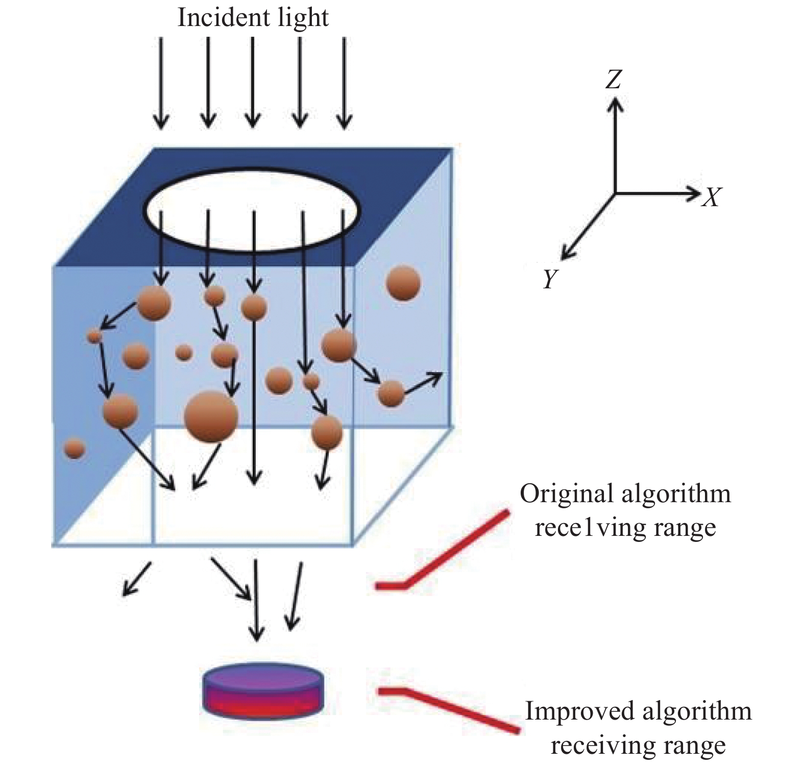
光波通过单个微粒,散射后能量分布沿不同方向呈现非均匀分布,S波和P波在不同角度的能量变化差异引起偏振态在不同角度分布不同。参照图1,当一束光经过散射介质,偏振子午面蒙特卡洛法计算过程中采集了全部前向散射光,但绝大部分接收装置仅能接收部分前向散射光。随着散射次数的增加,S波和P波在不同散射角度的偏振态分布差异不断富集,致使未采集的前向散射光与采集的前向散射光的偏振态通常存在差异,这是引起计算结果与测试结果存在差异乃至失配的重要因素,为此,改进算法对原算法的接收范围进行了限定。

图 1 偏振子午面蒙特卡洛法与改进算法的接收范围
Figure 1. Optical receiving range of polarization meridian Monte Carlo method and improved algorithm
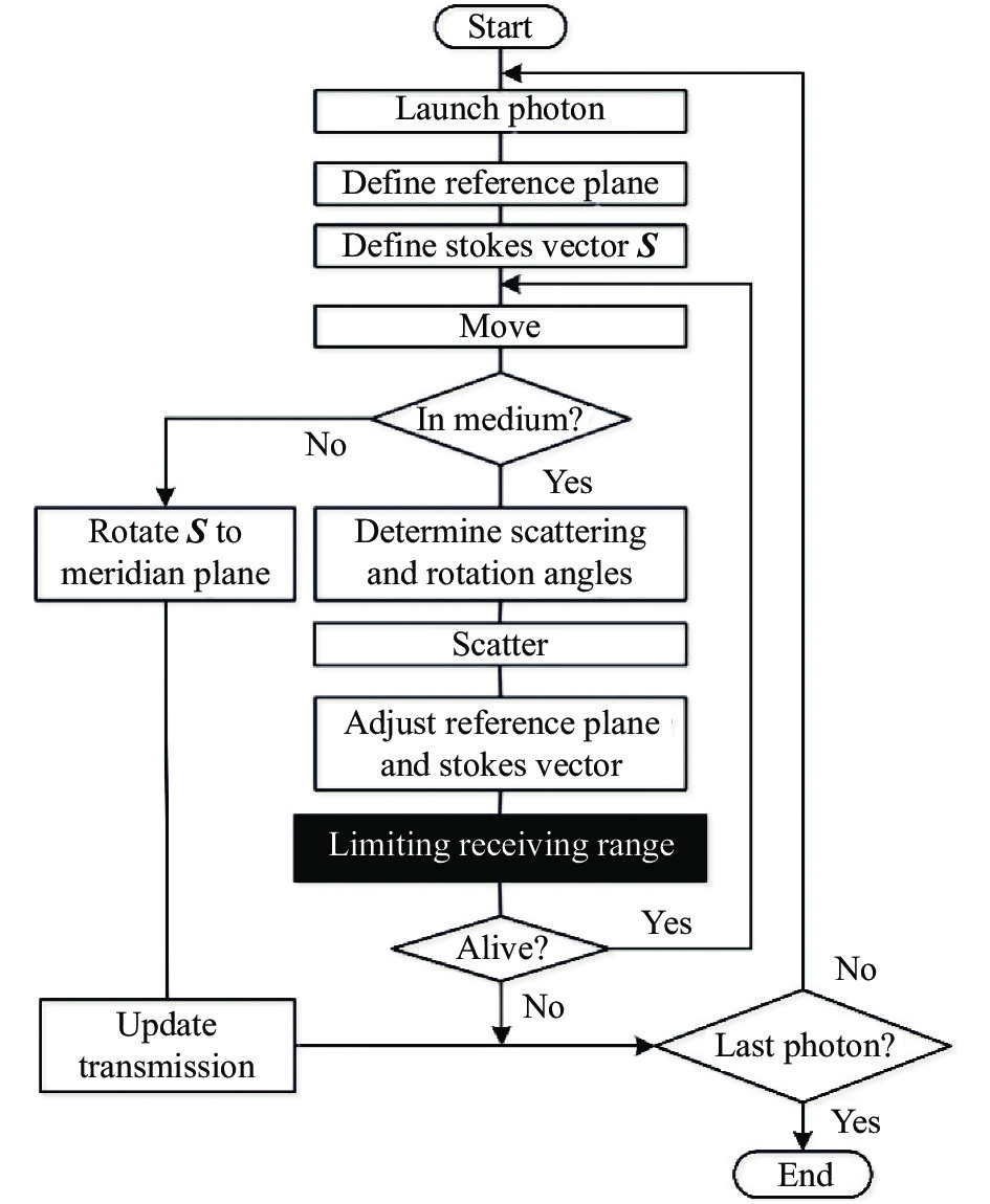
改进算法计算流程参照图2,灰框部分为改进算法增加的框图。改进算法的计算步骤为:发射光子,此时定义光子的初始参考平面;光子通过散射介质,由于吸收作用,光子会降低一些权重,由于散射作用,光子的偏振态旋转到新平面;判定光子是否在限定的接收范围内,如果超出限定接收范围则直接判定光子死亡;判定光子是否达到其他死亡条件,例如阈值过低;最后,通过“轮盘赌”算法,完成所有光子传输。

图 2 限定接收范围的改进算法流程图
Figure 2. Flow chart of the improved algorithm for limiting receiving range
改进算法相比偏振子午面蒙特卡洛法增加了限定接收范围的功能,设定的接收范围与实际探测器的接收范围一致。以平面接收装置为例描述设定过程:对于偏振子午面蒙特卡洛法,光子在真空介质经过预设距离后,将预设距离处垂直于光子初始传输方向的截面设定为接收平面;在该接收平面内,以预设距离处为中心,划定与实际探测器接收范围一致的区域,该区域则为限定的接收范围;发射光子于散射介质中,光子传输后判定光子是否在限定的接收范围内,如果光子在限定接收范围之外,则直接判定光子死亡。限定的接收范围还可按照实际检测装置面型开展设置,设置方法是在程序坐标系中设定与实际接收装置面型一致的图形,将其调整在预设距离处,通过判定光子是否经过限定的接收范围开展运算。
由于聚苯乙烯悬浊液是一种变量可控的散射环境,它能够提供较为理想的单分散体系环境,便于开展验证实验,为此,采用原算法和改进算法分别模拟水平线偏振光在聚苯乙烯悬浊液中传输。其中,波长设定为532 nm,聚苯乙烯悬浊液设置为粒径1 μm的单分散分布,其浓度分别设置为 1.04、2.08、4.17、8.33、12.50、16.67 μg/cm3。
-
聚苯乙烯悬浊液由聚苯乙烯原液与去离子水混合而成,原液的微粒粒径分为1 μm,原液的粒径标准差<5%,配置浓度分别为1.04、2.08、4.17、8.33、12.50、16.67 μg/cm3。配置后的聚苯乙烯悬浊液罐装于125 cm3的立方体石英玻璃容器中。入射光为532 nm波长的完全45°线偏振光或完全水平线偏振光,光在容器中的传输距离为5 cm。
为抑制外界和大角度前向散射光进入接收区域,对整个测试系统进行了相关设置。测试环境为黑布遮盖的密闭空间,测试时间为夜晚,避免了环境杂散光的干扰;聚苯乙烯悬浊液装配容器,除了前后方向之外,其余面均采用黑胶布覆盖,避免了一部分大角度前向散射光的外溢;实验开展于超净实验室中,环境经过除尘和除静电处理,确保环境干净,避免了空气中的杂质引起的散射;系统采用大口径物镜,而超出物镜接收范围的前向散射光被外围黑色遮布吸收,不会在环境中发生漫散射。
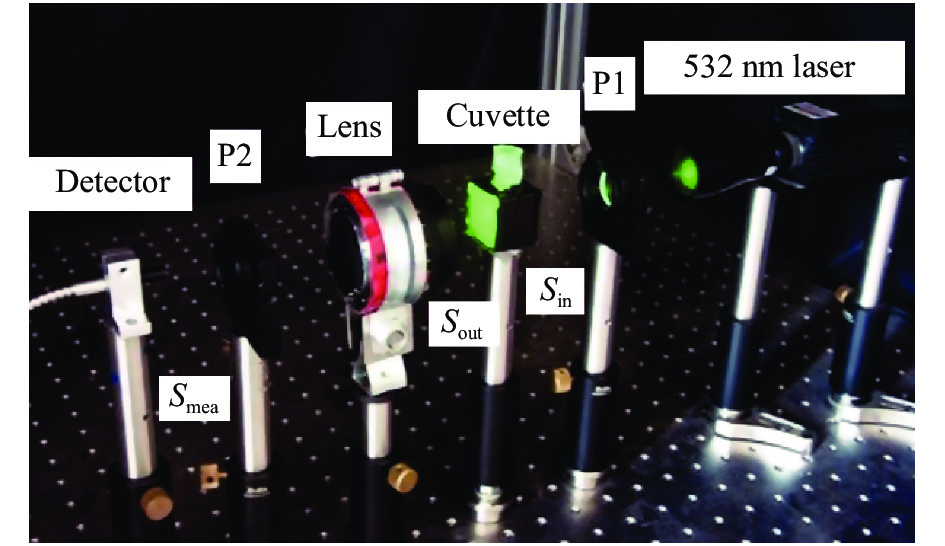
测试装置参照图3。532 nm激光通过偏振片P1转化为完全线偏振光Sin,线偏振光Sin通过聚苯乙烯悬浊液输出为Sout,之后由物镜收集,经由偏振片P2后获得Smea,最终由AvanSpec-ULS2048LTEC型光谱仪接收。

图 3 线偏振光传输实验装置
Figure 3. Experimental setup for linearly polarized light propagation
设聚苯乙烯悬浊液的穆勒矩阵为MP,Sout和Smea分别求解为:
$$ \boldsymbol{S}_{\rm{out}}=\boldsymbol{M}_{\rm{P}} \boldsymbol{S}_{\rm {in }} $$ (1) $$ \boldsymbol{S}_{\rm{mea}}={\boldsymbol P}_{2} \boldsymbol{M}_{\rm{P}} \boldsymbol{S}_{\rm{in}} $$ (2) 式中:P2代表米勒矩阵。公式(2)转化为:
$$ \left[\begin{array}{l} S_{0 \rm{mea}} \\ S_{1 \rm{mea}} \\ S_{2 \rm{mea}} \\ S_{3 \rm{mea}} \end{array} \right]=\left[\begin{array}{cccc} 1 \;\;\cos 2 {\rm {\theta}} \;\;\sin 2 {\rm {\theta}} \;\;0 \\ \cos 2 {\rm {\theta}} \;\;\cos ^{2} 2 {\rm {\theta}} \;\;\sin 2 {\rm {\theta}} \cos 2 {\rm {\theta}} \;\;0 \\ \sin 2 {\rm {\theta}} \;\;\sin 2 {\rm {\theta}} \cos 2 {\rm {\theta}} \;\;\sin ^{2} 2 {\rm {\theta}} \;\;0 \\ 0 \;\;0 \;\;0 \;\;0 \end{array}\right] \\ \cdot \frac{1}{2}\left[\begin{array}{c} S_{0 \rm { out }} \\ S_{1 \rm { out }} \\ S_{2 \rm { out }} \\ S_{3 \rm { out }} \end{array}\right] $$ (3) 将公式(3)展开得:
$$ \begin{split} 2 S_{0 \rm { mea }}= &S_{0 \rm { out }}+S_{\rm {1out }} \cos 2 {\rm {\theta}}+S_{2 \rm { out }} \sin 2 {\rm {\theta}} \\ 2 S_{1 \rm { mea }}= &S_{0 \rm { out }} \cos 2 {\rm {\theta}}+S_{1 \rm { out }} \cos ^{2} 2 {\rm {\theta}}+ \\ &S_{2 \rm { out }} \sin 2 {\rm {\theta}} \cos 2 {\rm {\theta}} \\ 2 S_{2 \rm { mea }} =&S_{0 \rm { out }} \sin 2 {\rm {\theta}}+S_{\rm {1out }} \sin 2 {\rm {\theta}} \cos 2 {\rm {\theta}} +\\ &S_{2 \rm { out }} \sin ^{2} 2 {\rm {\theta}} \end{split} $$ (4) 公式(4)中有 3 个待求参数,通过测量偏振片旋转至不同角度下的 3 组光强值即可求解,求解后得到 Sout。
为了求解聚苯乙烯悬浊液的穆勒矩阵,需选择4种不同的偏振光作为输入光,入射光分别设置为 Sin−1、Sin−2、Sin−3、Sin−4,求解输出光分别为Sout−1、Sout−2、Sout−3、Sout−4。分别建立秩为 4 的输入矩阵和输出矩阵,输入矩阵和输出矩阵之间关系为:
$$ \left[\boldsymbol{S}_{\rm {out }-1}, \boldsymbol{S}_{\rm {out- } 2}, \boldsymbol{S}_{\rm {out }-3}, \boldsymbol{S}_{\rm {out- } 4}\right] \\ =\boldsymbol{M}_{\rm{p}}\left[\boldsymbol{S}_{\rm{in}-1}, \boldsymbol{S}_{\rm{in}-2}, \boldsymbol{S}_{\rm{in}-3}, \boldsymbol{S}_{\rm{in}-4}\right] $$ (5) 求解聚苯乙烯悬浊液的穆勒矩阵 Mp为:
$$ \boldsymbol{M}_{\rm{p}}=\left[\boldsymbol{S}_{\rm {out- } 1}, \boldsymbol{S}_{\rm {out- } 2}, \boldsymbol{S}_{\rm {out- } 3}, \boldsymbol{S}_{\rm {out-4 }}\right] \\ ·\left[\boldsymbol{S}_{\rm{in}-1}, \boldsymbol{S}_{\rm{in}-2}, \boldsymbol{S}_{\rm{in}-3}, \boldsymbol{S}_{\rm{in}-4}\right]^{-1} $$ (6) -
由于偏振度计算过程不仅引入了初始入射光的正交分量光强,而且掺杂着具有其他偏振态光波的光强,评估时缺乏一定的精度。偏振状态保持率(Retention rate of polarization state,RoPS)[15-16]用于表征前向散射光中与初始入射光具有相同偏振态的光波光强占前向散射光总光强的比例,它不仅能够规避正交分量光强度差值计算所引入的误差,而且规避了其他偏振态光强的影响,因此,采用RoPS作为评估指标。其中,RoPS可由穆勒矩阵元素求得,具体求解过程参考文献[16]。
当 45°线偏振光前向传输时,RoPS 表达为:
$$ R o P S_{\rm {light-45 }}=\frac{P_{45 \rm {-out-forward }}}{P_{0 \rm {-out-forward }}} $$ (7) 式中:P0-out-forward表示前向散射光的总光强度;P45-out-forward代表前向散射光中45°线偏振光的光强度。
当水平线偏振光前向传输时,RoPS表达为:
$$ R o P S_{\rm {light-H }}=\frac{P_{\rm {H-out-forward }}}{P_{0 \rm {-out-forward }}} $$ (8) 式中:P0-out-forward表示前向散射光的总光强度;PH-out-forward代表前向散射光中水平线偏振光的光强度。
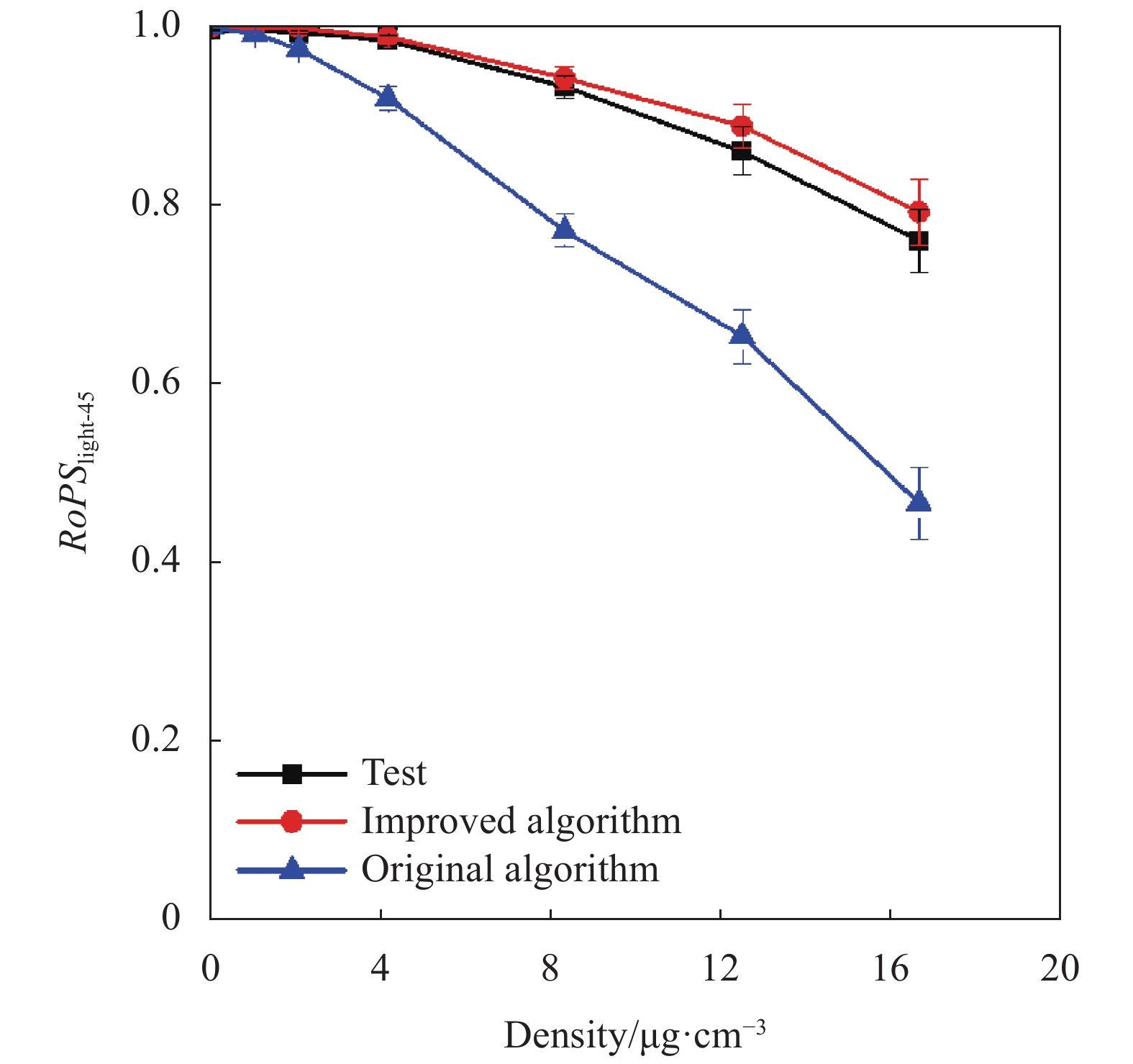
图4显示了 45°线偏振光在聚苯乙烯悬浊液中前向传输的计算和测试结果,重复模拟计算和实验测试 5 次以确保结果的准确性。结果显示:随着浓度的增加,偏差范围基本呈现逐渐增加的趋势;且在低浓度条件下,改进算法与原算法计算差异较小,随着浓度的增加,改进算法较原算法更贴近实测结果。结果表明:在较高浓度的聚苯乙烯悬浊液中,改进算法的计算结果相比偏振子午面蒙特卡洛法更接近测量值。
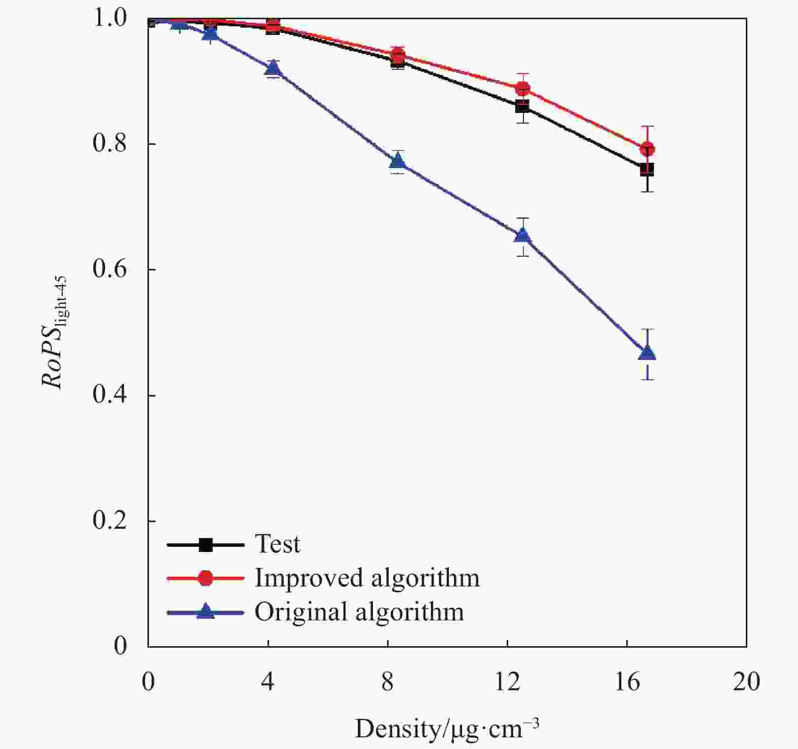
图 4 45°线偏振光在聚苯乙烯悬浊液中前向传输的改进算法、原算法与实测结果
Figure 4. Improved algorithm, original algorithm and measured results of 45° linearly polarized light propagating in polystyrene suspension
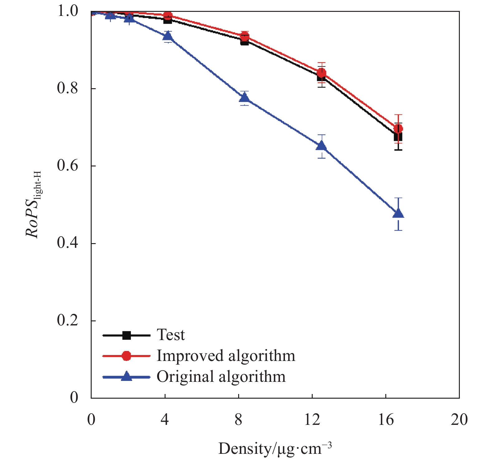
图5显示了水平线偏振光在聚苯乙烯悬浊液中前向传输的计算和测试结果,重复模拟计算和实验测试5次以确保结果的准确性。结果显示:随着浓度的增加,偏差范围基本呈现逐渐增加的趋势;且在低浓度条件下,改进算法与原算法计算差异较小,随着浓度的增加,改进算法较原算法更贴近实测结果。结果表明:在较高浓度的聚苯乙烯悬浊液中,改进算法的计算结果相比偏振子午面蒙特卡洛法更接近测量值。

图 5 水平线偏振光在聚苯乙烯悬浊液中前向传输的改进算法、原算法与测试结果
Figure 5. Improved algorithm, original algorithm and measured results of horizontally linearly polarized light propagating in polystyrene suspension
统观45°线偏振光和水平圆偏振光在聚苯乙烯悬浊液中前向传输的计算结果和测试结果,得出结论:相比偏振子午面蒙特卡洛法,改进算法的计算结果与测试结果更为匹配。
-
求解45°线偏振光通过单个聚苯乙烯微球后全部前向散射角的RoPSlight-45分布。计算结果参照图6,[−90°,90°]区间覆盖全部前向传输范围,这与原算法的接收范围是等价的。计算结果显示:RoPSlight-45数值在[−90°, 25°]和[25°, 90°]区间内波动明显,RoPSlight-45数值在 [−25°, 25°]区间内略有波动。计算结果表明:在[−90°, −25°]和[25°, 90°]区间内偏振状态产生一定变化,在[−25°, 25°]区间内偏振状态变化很小。随着散射次数的增加,原算法中前向散射角外延程度较大的散射光不断富集,致使原算法的计算结果偏离测试结果,而改进算法规避了绝大部分前向散射角外延程度较大的散射光,致使改进算法的计算结果更接近测试结果。

图 6 单个微粒的RoPSlight-45随前向散射角的分布
Figure 6. RoPSlight-45 distribution of individual particle versus forward scattering angles
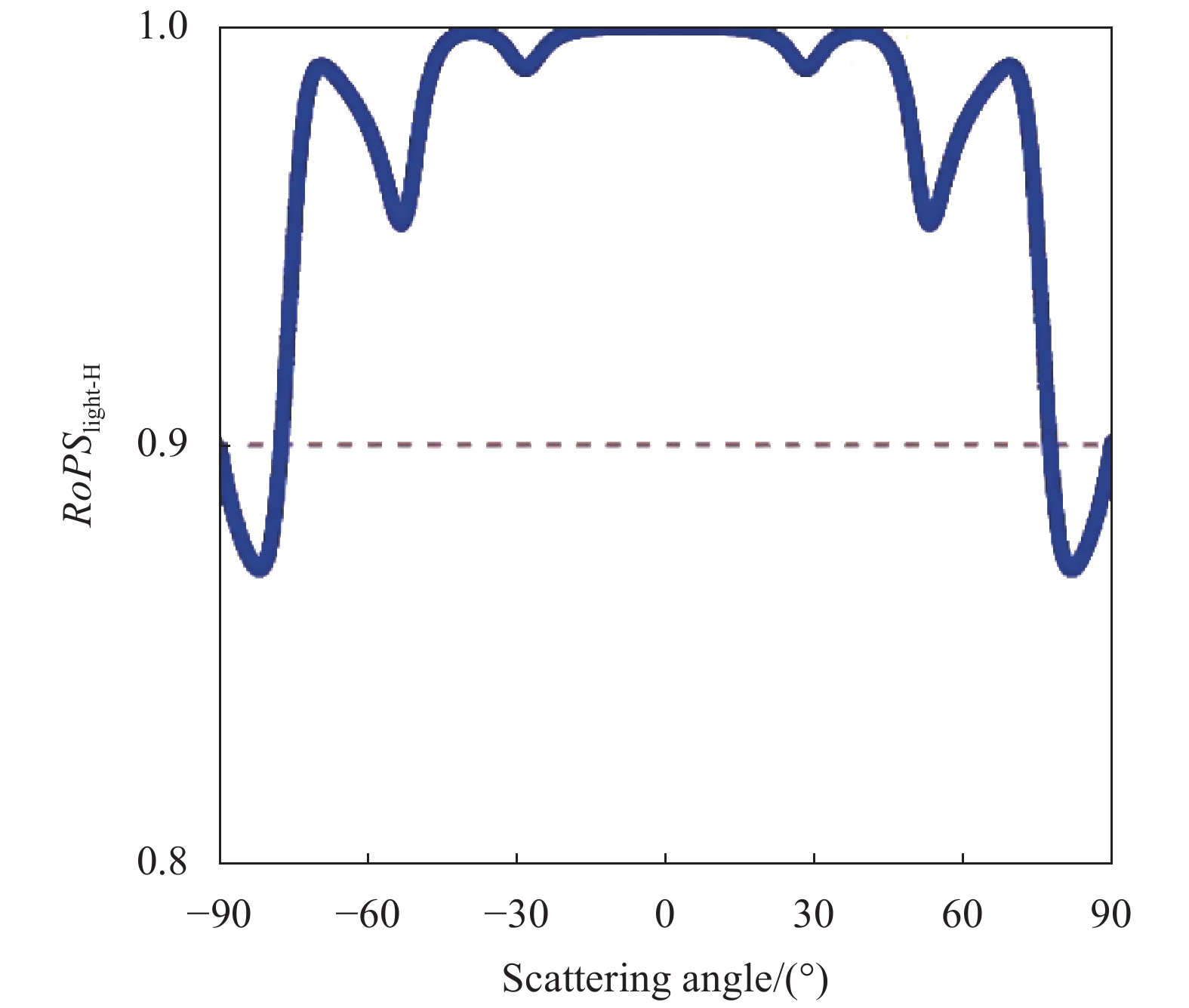
求解水平线偏振光在单个聚苯乙烯微球中前向传输的RoPSlight-H分布。计算结果参照图7,计算结果显示:RoPSlight-H数值在[−90°, −40°]和[40°, 90°]区间内波动明显,在[−40°,40°]区间内略有波动。计算结果表明:在[−90°,−40°]和[40°, 90°]区间内传输光的偏振状态产生一定变化,在区间[−40°,40°]内传输光的偏振状态变化很小。多次散射使得原算法中前向散射角外延程度较大的散射光不断富集,导致原算法的计算结果偏离测试结果,而改进算法规避了绝大部分前向散射角外延程度较大的散射光,这使得改进算法的计算结果更接近测试结果。

图 7 单个微粒的RoPSlight-H随散射角的分布
Figure 7. RoPSlight-H distribution of individual particle versus scattering angles
-
为弥补偏振子午面蒙特卡洛法的计算结果与测试结果存在出入的问题,解决由模拟方法所导致的偏振子午面蒙特卡洛法与实验环境的测试结果存在出入的问题,文中提出了一种限定接收范围的改进算法。改进算法增加了限定前向散射光的接收范围的功能,且限定的接收范围与实际接收范围一致。选用参量可控的聚苯乙烯悬浊液开展计算和测试,采用原算法和改进算法分别模拟完全 45°线偏振光和完全水平线偏振光在聚苯乙烯悬浊液中的前向传输特性,并通过实验验证了改进算法比原算法能够更好的匹配实测结果。计算单个微粒的偏振状态保持率,分析了改进算法提高计算精度的作用机理,即随着前向散射角外延,散射光的偏振态变化愈剧烈,而改进算法规避了绝大部分前向散射角外延程度较大的散射光。文中研究能为偏振光前向传输量化实验的精确测量提供算法支持。此外,由于改进算法是基于前向散射偏振态变化的特性,对于后向散射的情形,后续研究尚需从理论和算法方面拓展,以期完善改进算法的适用范围。
Optimized algorithm to limit receiving range of polarized light forward propagation into scattering media
-
摘要: 为解决偏振子午面蒙特卡洛法的计算结果与测试结果存在出入的问题,文中提出了一种限定接收范围的改进算法。偏振子午面蒙特卡洛法计算过程中采集整个截面的前向散射光,但实际接收装置通常接收部分前向散射光,这是引起偏振子午面蒙特卡罗法的计算结果与实验结果存在出入乃至失配的重要因素之一。为此,改进算法限定了前向散射光的接收范围,限定的接收范围与实际接收范围一致。采用原算法和改进算法分别模拟 45°线偏振光和水平线偏振光在聚苯乙烯悬浊液中传输。选用粒径 1 μm 的聚苯乙烯悬浊液开展验证实验,通过对照测试结果,改进算法相比原算法能够更好地匹配实测结果。通过计算单个微粒的偏振状态保持情况,阐明改进算法提高计算精度的作用机理,即前向散射角愈外延,散射光的偏振态变化愈剧烈,而改进算法规避掉了绝大部分前向散射角外延程度较大的散射光。Abstract: To solve the problem of discrepancies between calculation results and test results of the polarization meridian Monte Carlo method, an improved algorithm which can limit receiving range was proposed. All forward scattered light was received generally in real receiving devices in the process of calculation, but part of forward scattered light was collected. This is one of the important factors causing discrepancies and mismatch between calculation results and test results of the polarization meridian Monte Carlo method. For this reason, an improved algorithm was proposed to limit receiving range of forward scattered light. Receiving range of the improved algorithm was consistent with real receiving range. Original algorithm and improved algorithm were used to simulate the propagation of 45°- and horizontally- linearly polarized light in polystyrene suspension, respectively. Then, the polystyrene suspension with particle size of 1 μm were selected to carry out verification experiments. Compared with the original algorithm, simulation results of the improved algorithm were closer to measured values. Finally, the polarization state distribution of a single particle was calculated to clarify mechanism of improved accuracy. Retention of polarization state(RoPS) changes drastically as forward scattered angle extends. Improved algorithm avoids most of forward scattered light with larger forward scattered angles.
-
图 1 偏振子午面蒙特卡洛法与改进算法的接收范围
Figure 1. Optical receiving range of polarization meridian Monte Carlo method and improved algorithm
图 2 限定接收范围的改进算法流程图
Figure 2. Flow chart of the improved algorithm for limiting receiving range
图 4 45°线偏振光在聚苯乙烯悬浊液中前向传输的改进算法、原算法与实测结果
Figure 4. Improved algorithm, original algorithm and measured results of 45° linearly polarized light propagating in polystyrene suspension
图 5 水平线偏振光在聚苯乙烯悬浊液中前向传输的改进算法、原算法与测试结果
Figure 5. Improved algorithm, original algorithm and measured results of horizontally linearly polarized light propagating in polystyrene suspension
图 6 单个微粒的RoPSlight-45随前向散射角的分布
Figure 6. RoPSlight-45 distribution of individual particle versus forward scattering angles
-
[1] Sankaran V, Walsh J T, Maitland D J. Polarized light propagation through tissue phantoms containing densely packed scatterers [J]. Optics Letters, 2000, 25(4): 239-241. doi: 10.1364/OL.25.000239 [2] Zeng X W, Chu J K, Cao W D, et al. Visible–IR transmission enhancement through fog using circularly polarized light [J]. Applied Optics, 2018, 57(23): 6817-6822. doi: 10.1364/AO.57.006817 [3] Fade J, Panigrahi S, Carre A, et al. Long-range polarimetric imaging through fog [J]. Applied Optics, 2014, 53(18): 3854-3865. doi: 10.1364/AO.53.003854 [4] Guo Z Y, Wang X Y, Li D K, et al. Advances on theory and application of polarization information propagation(Invited) [J]. Infrared and Laser Engineering, 2020, 49(6): 20201013. (in Chinese) doi: 10.3788/IRLA20201013 [5] Collin C, Pattanaik S, LiKamWa P, et al. Discrete ordinate method for polarized light transport solution and subsurface BRDF computation [J]. Computers & Graphics, 2014, 45: 17-27. [6] Tapimo R, Kamdem H T T, Yemele D. A discrete spherical harmonics method for radiative transfer analysis in inhomogeneous polarized planar atmosphere [J]. Astrophysics and Space Science, 2018, 363(3): 52. doi: 10.1007/s10509-018-3266-5 [7] Zhang Y, Zhang Y, Zhao H J. A skylight polarization model of various weather conditions [J]. Journal of Infrared and Millimeter Waves, 2017, 36(4): 453-459. (in Chinese) doi: 10.11972/j.issn.1001-9014.2017.04.013 [8] Ramella-Roman J C, Prahl S A, Jacques S L. Three Monte Carlo programs of polarized light transport into scattering media: Part I [J]. Optics Express, 2005, 13(12): 4420-4438. doi: 10.1364/OPEX.13.004420 [9] Markel V A. Two-stream theory of light propagation in amplifying media [J]. JOSA B, 2018, 35(3): 533-544. doi: 10.1364/JOSAB.35.000533 [10] Ven der laan J D, Wright J B, Scrymgeour D A, et al. Variation of linear and circular polarization persistence for changing field of view and collection area in a forward scattering environment[C]//International Society for Optics and Photonics, 2016. [11] Ven der laan J D, Wright J B, Scrymgeour D, et al. Effects of collection geometry variations on linear and circular polarization persistence in both isotropic-scattering and forward-scattering environments [J]. Applied Optics, 2016, 55(32): 9042-9048. doi: 10.1364/AO.55.009042 [12] Ven der laan J D. Evolution and persistence of circular and linear polarization in scattering environments[D]. Tucson: University of Arizona, 2015. [13] Slade W H, Agrawal Y C, Mikkelsen O A. Comparison of measured and theoretical scattering and polarization properties of narrow size range irregular sediment particles[C]//IEEE, 2013. [14] Ghosh N, Gupta P K, Patel H S, et al. Depolarization of light in tissue phantoms – effect of collection geometry [J]. Optics Communications, 2003, 222(1): 93-100. [15] Zeng X W, Chu J K, Wu Q M, et al. Polarization state persistence characteristics in wet haze within PM2.5 for forward transmission[C]//2019 International Conference on Optical Instruments and Technology: Optical Communication and Optical Signal Processing, 2020, 11435: 1143509. [16] Chu J K, Wu Q M, Zeng X W, et al. Forward transmission characteristics in polystyrene solution with different concentrations by use of circularly and linearly polarized light [J]. Applied Optics, 2019, 58(25): 6750-6754. doi: 10.1364/AO.58.006750 -

 点击查看大图
计量
- 文章访问数: 240
- HTML全文浏览量: 94
- PDF下载量: 22
- 被引次数: 0


