In the field of optical microscopy, phase research provides information such as depth and refractive index for biological cells and other objects, which has become an important reference index. At the same time, the solution method of phase is also widely concerned. Among them, the non-interference phase retrieval method based on the Transport of Intensity Equation (TIE) has been applied to microscopic fields, such as living cell detection^[1], red blood cell detection^[2], breast cancer cell quantitative imaging^[3], etc, because it solves the equation directly through the intensity image to obtain the phase, does not need complicated calculation and devices, and reduces coherent noise^[4-6].

When solving TIE, it is necessary to obtain the focus image and the corresponding defocus images along the optical axis direction^[7-8]. In actual operation, a series of intensity images are usually obtained along the optical axis direction. But it is impossible to determine whether focus images are included in the collected images. In the case of containing the focus image, simple subjective identification can not find the optimal focus position, thus affect the accuracy of phase retrieval. In the case of not containing the focus image, it is often necessary to locate the position of the focus image through the acquisition of a large number of images again, which leads to the complicated process of phase solution. As for the positioning of microfocus images, many experts and scholars have made hardware modifications. Mao Bangfu of Zhejiang University^[9] designed a microscopic automatic focusing system. The system drives the micro-handwheel of the microscope rotation through a stepping motor, which makes the stage move up and down to realize the function of automatic focusing. However, this modification requires complicated devices and high cost. Yu Yang et al.^[10] of Nanjing University of Aeronautics and Astronautics have designed a microscope hardware auto-focusing system based on photoelectric position sensitive detector (PSD), which can control the displacement in the z-axis direction of the automatic microscope system in real time. It also improves the auto-focusing capability of the microscope. However, the input-output linearity of the hardware system is not accurate and needs linear compensation.

In terms of software, Tian Xiaolin et al.^[11] of Jiangnan University used cell duty ratio to judge the in-focus images, which judges image focus by calculating the area ratio of the sample to the background. But for continuous samples, it is impossible to distinguish between the sample and the background. So this method is only applicable to discrete samples. Cheng Hong et al.^[12] of Anhui University proposed an transport of intensity equation algorithm(EDR-TIE) based the edge detection and duty ratio, which expanded the application range of samples. However, this method requires the collected image sequence to contain the focus image, and the position of the focus image is determined through one-time positioning by the algorithm. When there is no focus image in the collected image sequence, the algorithm cannot accurately locate. On this basis, this paper proposed a phase retrieval algorithm (AF-TIE) based on the transport of intensity equation under adaptive focus. This algorithm locates the reference focus position by edge duty ratio from the original image sequence, and then uses the reference focus image to calculate the focus position. It is suitable for discrete samples and continuous samples, and there is no restriction on whether the focus image is contained or not.

In a coherent light field, assuming that monochromatic light propagates along the z-axis under the condition of paraxial approximation. Teague deduced the transport of intensity equation^[13], which can be expressed as:

Among them, ${{\textit{z}}_0}$ is the propagation distance, $\lambda $ is wavelength, $I(x,y,{{\textit{z}}_0})$ and $\phi (x,y,{{\textit{z}}_0})$ are the intensity and phase of the object on the focus plane, $\nabla {\rm{ = }}({\partial _x},{\partial _y})$ is the gradient operator on the plane of $x - y$, $\partial I(x,y,{\textit{z}})/\partial z$ represents the amount of variation in the intensity distribution along the axis, i.e. intensity differential, which cannot be measured directly and is usually estimated by using finite difference. Assuming the $I(x,y,{{\textit{z}}_0}{\rm{ + }}\Delta {\textit{z}})$ and $I(x,y,{{\textit{z}}_0} - \Delta z)$ are the over-focus intensity image and the under-focus intensity image when the defocus distance is $\Delta {\textit{z}}$, as shown in Fig.1. The intensity differential can be zapproximately estimated by Eq.(2):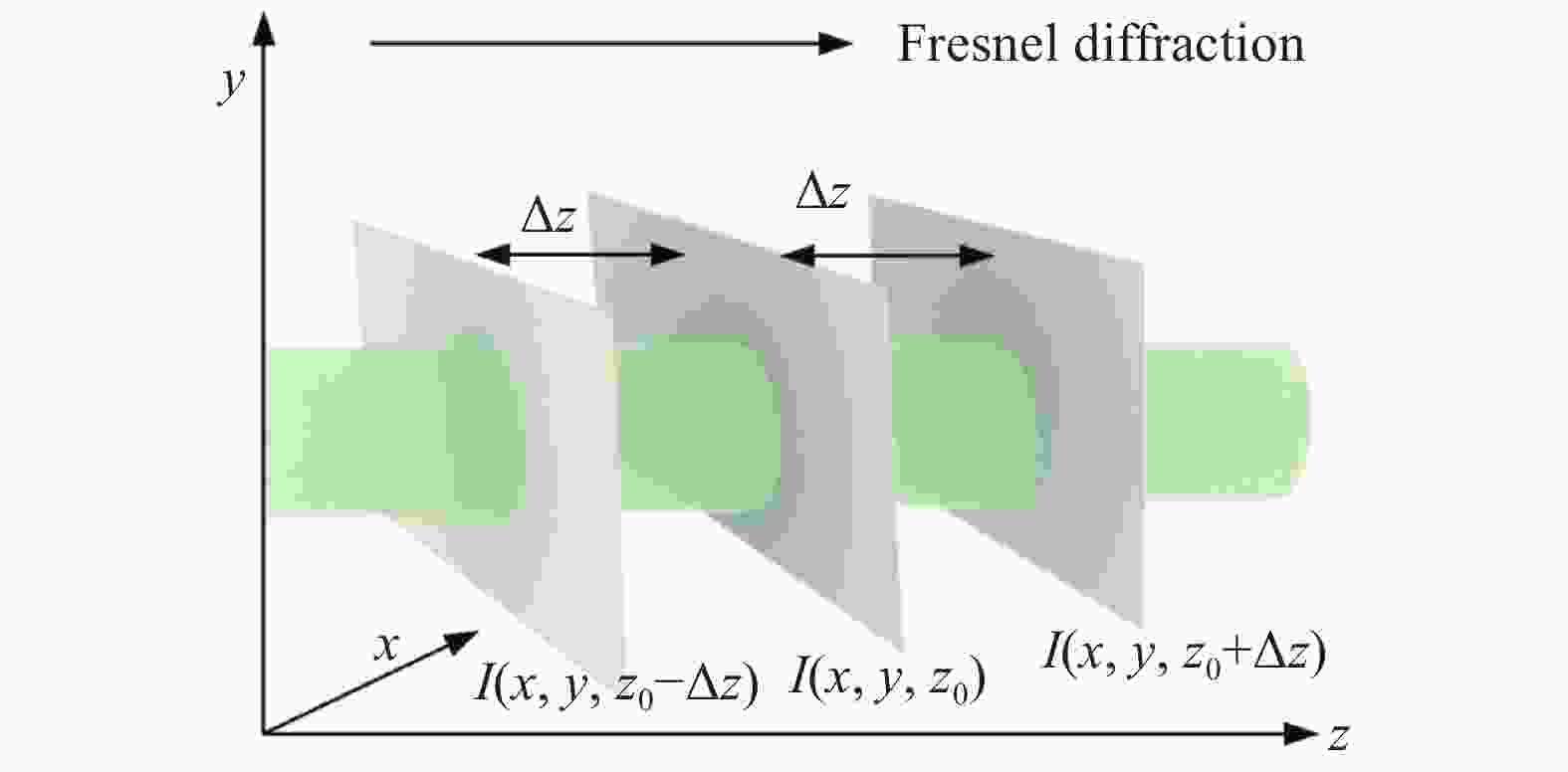

Figure 1.  Schematic diagram of intensity differential estimation

Substitute Eq.(2) into Eq.(1) can be obtained:

The only unknown quantity $\phi (x,y,{{\textit{z}}_0})$ can be obtained through Eq.(3).

In microscopic imaging, the built-in LED light wave used is partially coherent. The corresponding ${\phi _{out}}(x,y,{{\textit{z}}_0})$ is a generalized phase, which consists of the phase of the illumination light ${\phi _{in}}(x,y,{{\textit{z}}_0})$ and the phase of the object $\phi (x,y,{{\textit{z}}_0})$, i.e.

Because the microscope satisfies the infinity correction optical system, i.e. the telecentric optical path. At the same time, using symmetrical Kohler illumination in the microscope, which satisfy the zero distance condition. Therefore, the phase of partially coherent light is consistent with that of traditional objects, and the corresponding generalized TIE is completely consistent with that of completely coherent illumination. Therefore, the traditional TIE phase retrieval method can be directly used to solve the phase of the object under the partially coherent light field in the microscope^[14].

As shown in Eq.(3), the accurate selection of the focus image will affect the accuracy of phase retrieval. The edge duty ratio positioning method can help focus determination. the edge duty ratio is shown in Eq.(5)^[12]:

${N_T}$ is the total number of pixels of the picture, ${N_B}$ indicate the corresponding edge information point pixels of the object.

In this paper, the Prewitt operator is used to extract the edge information of the image. The neighborhood pixel gray value of the image function $f\left( {x,y} \right)$ at point $\left( {i,j} \right)$ is showed in Fig.2(a). Fig.2(b) and Fig.2(c) are the Prewitt operator template of horizontal and the vertical respectively. The gradient amplitude $\nabla f$ and first derivative $g$ are shown in Eq.(6):

Figure 2.  Edge detect. (a) The gray value of the image's neighborhood pixel at （i,j）; (b) Prewitt operator level template ; (c) Prewitt operator vertical template

Duty ratio as the evaluation standard of focus image, which is the area ratio of the sample to the background in the image actually. When the collected intensity map is located in the focused plane, the target sample occupies the least area in the image. If the position deviates from the focal plane, halos will appear under the influence of diffraction effect, blurring the sample boundary, thus increasing the proportion of sample edge information in the whole image area. With the increase of defocus distance, the proportion of edge information will be larger. Therefore, the focus intensity image can be judged by calculating the number of pixels occupied by the sample edge, that is to say the focus position can be located from a series of intensity maps by using the characteristic of "the duty ratio of the optimal focus image is the minimum"^[9].

When the collected image sequence contains focus image, the EDR-TIE algorithm proposed in reference[12] can be used directly to detect the optimal focused position. However, when the focus image is not included, use the EDR-TIE algorithm directly can only be used to locate in the first or the last position of this column of intensity images. So, in order to obtain the focus position, we need to collect a large number of images again. Based on EDR-TIE, this paper proposes an positioning method of adaptive focusing, i.e. AF-TIE algorithm, and its flow chart is shown in Fig.3.

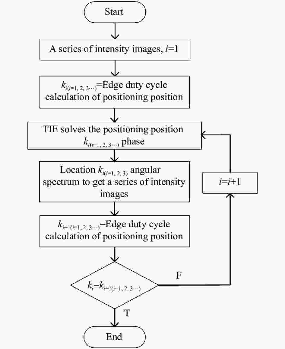
Figure 3.  Algorithm flow chart

Firstly, the edge duty ratio method is used to locate k₁ position through a series of existing intensity images, and the phase at k₁ position can be solved by TIE, which used intensity image and corresponding defocus images. The phase and intensity form a wavefront. Then use the angular spectrum propagation to obtain a new series of intensity images. The edge duty ratio is used to detect and locate, and the position is found to be k₂. If k₁ and k₂ are equal, k₁ is considered to be the optimal focus position, and the focus image are considered to be contained in the series of intensity maps. If k₁ and k₂ are not equal, the intensity image and the corresponding defocus images of k₂ position are obtained. So the phase of k₂ position is solved, and a new series of intensity images are obtained by angular spectrum propagation again. Continue to postion with edge duty cycle, compare and cycle until the position obtained by positioning is no longer changed, ending the cycle.

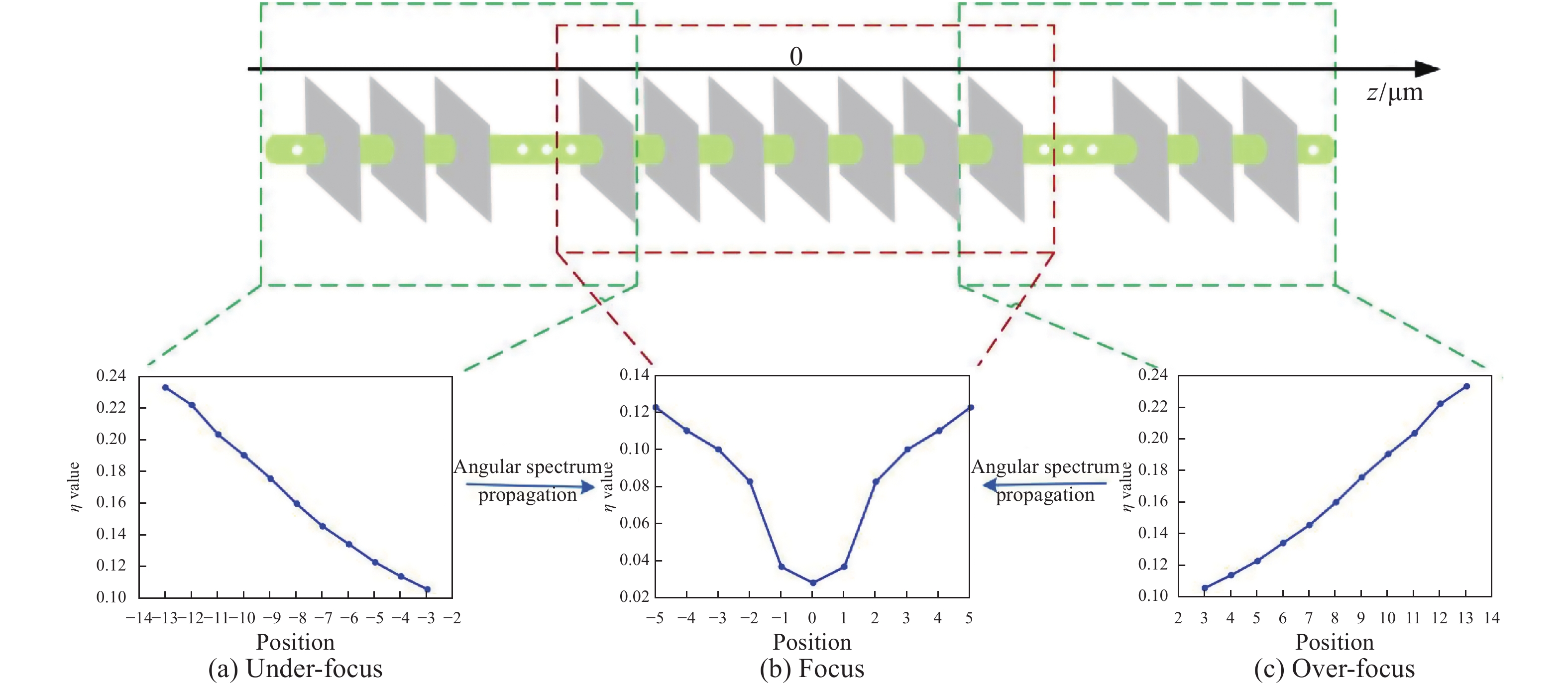
In the above angular spectrum propagation, we all choose one-direction propagation, because if the collected series of intensity images contain focus image, as shown in Fig.4(b). The positioning position does not change after the first positioning and the angular spectrum propagation in one direction. If the focus image is not included, this series of intensity images can only be on the under-focus side or on the over-focus side, as shown in Fig.4(a) and Fig.4(c). After the edge duty ratio is positioned. We choose to propagate the angular spectrum to the side with small edge duty ratio, that is, to the side with focus.

Figure 4.  Schematic diagram of edge duty ratio and angular spectrum propagation direction under different conditions

Assuming that the optimal focus position is at ${\textit{z}}_0'$, then the defocus image $I(x,y,{\textit{z}}_{_0}' + \Delta z)$ and $I(x,y,{\textit{z}}_{_0}' - \Delta z)$ are selected at the position ${\textit{z}}_{_0}' \pm \Delta {\textit{z}}$, and the Eq.(2) is used to obtain the following formula

Allen et al. proposed that the solution of Eq.(1) can be obtained by Fourier operator step-by-step calculation. Set

For any function $f(x,y)$, its Fourier properties can be described as:

In the formula, $x$ and $y$ respectively represents the vector of $x$ and $y$ direction, $F$ is Fourier transform, ${F^{ - 1}}$ is inverse Fourier transform and $({f_x},{f_y})$ is spatial frequency coordinate. Combining Eq.(8) and Eq.(10) to obtain:

The value of the phase is obtained by using Fourier properties again, which can be expressed as:

In this section, simulation experiments are carried out on the collected image sequence with focus and without focus respectively.

Firstly, the simulated experimental samples are selected. The intensity and phase images of the focus plane are shown in Fig.5(a) and Fig.5(b) respectively. The simulated image size is set to 256×256 pixel. Setting the focus position to 0 position. Firstly, five defocus images are obtained respectively before and after the focus plane by angular spectrum propagation, as shown in Fig.5(c). EDR-TIE algorithm is used directly for 11 intensity images which include focus image. The edge duty ratio detection results are shown in Fig.5(d), and it can be found that the focus image located at 0 position. The phase solution is carried out by the intensity image and the corresponding defocus images where the 0 position is located, and the result is shown in Fig.5(d).

Figure 5.  Simulation experiment. (a) Set intensity image; (b) Set phase image; (c) A series of intensity images (including focus) of angular spectrum propagation; (d) EDR-TIE positioning calculation results and 0 position phase results graph; (e) AF-TIE positioning calculation result graph

The cycle operations continue to carry out by the AF-TIE algorithm. Using the intensity image of the 0 position and the phase image obtained by the solution to do angular spectrum propagate to the in-focus side, thus 11 intensity images are obtained, then the edge duty ratio detection is carried out again. If it found that the position is consistent with which obtain by EDR-TIE algorithm, as shown in Fig.5(e). Therefore, the 0 postion is considered as the optimal focus position which matches the set focus position.

Assuming that the original phase is $\phi $, the retrieved phase is ${\phi _r}$. Define error formula as^[15]:

The error of the phase result between the optimal focus position and the set position is 0.3050. It can be seemed that both EDR-TIE and AF-TIE algorithm proposed in this paper can locate the optimal focus position when the focus image is included.

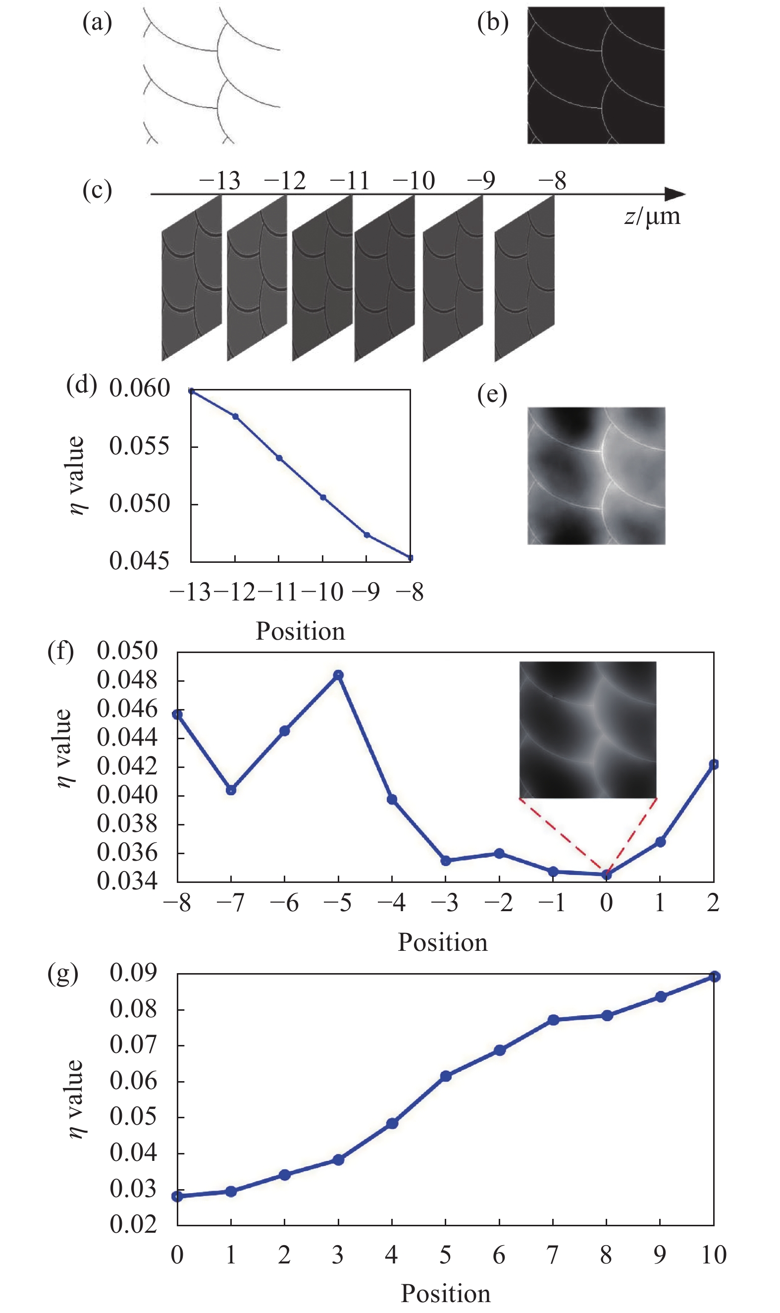
The intensity and phase in the focus plane of the simulated experimental sample are shown in Fig.6(a) and Fig.6(b) respectively. The distance between the two adjacent images is 100 μm, 0 position is the real focus position, and defocus images at positions from −8 to −13 are obtained by angular spectrum propagation, as shown in Fig.6(c). There is no focus image in this series of images. EDR-TIE algorithm is directly calculated from these 6 images. The positioning result is shown in Fig.6(d), and it can be found that it is located at the position of −8. We use angle spectrum by images at −8 position to obtain the intensity at −7 position. Then, using the intensity images at positions −9, −8, and −7 to obtain the phase of −8 position through TIE and the result is shown in Fig.6(e). Obviously, the EDR-TIE positioning result is inaccurate. If we want to obtain the focus image further, we usually need to collect a large number of intensity images again. Using AF-TIE algorithm in this paper, unidirectional angular spectrum propagation and edge duty ratio detection are carried out from the intensity image and the phase image at −8 position obtained by solution, and it is found that the focus plane is located at 0 position. The result is shown in Fig.6(f). Then move the translation table to collect the intensity image and the corresponding defocus images in 0 position, and the phase result show in Fig.6(f). Once again, one-directon angular spectrum propagation and edge duty ratio calculation are carried out to obtain the result in Fig.6(g), and it is found that it is located at its own position. Therefore, the 0 position is the optimal focus position, which is also the preseted. Then ending the cycle. This process reduce the collection number of intensity images.

Figure 6.  Simulates experiment. (a) Set intensity image; (b) Set phase image; (c) A series of intensity images (unfocused) of angular spectrum propagation; (d) EDR-TIE positioning calculation results; (e) Phase retrieval results of EDR-TIE positioning positions; (f) AF-TIE positioning calculation results and phase retrieval results; (g) A series of intensity image AF-TIE positioning calculation results propagated by the 0 position angular spectrum in Fig.6(f)

In order to further compare the phase results of EDR-TIE algorithm and AF-TIE algorithm, an image quality evaluation index SSIM (structural similarity index) is introduced to measure the image structural similarity^[16].

With the two images $X$ and $Y$ entered, ${\mu _X}$ and ${\mu _Y}$ represent the average of $X$ and $Y$, ${\sigma _X}$ and ${\sigma _Y}$ represent the standard deviation of $X$ and $Y$, ${\sigma _{XY}}$ is the covariance of $X$ and $Y$, ${C_1}$ and ${C_2}$ are the constants.

The error and similarity between the phase results of EDR-TIE algorithm and AF-TIE algorithm and the set phase are calculated by Eq.(13) and Eq.(14) respectively, as shown in Tab.1. The effectiveness and accuracy of the algorithm proposed in this paper are proved.

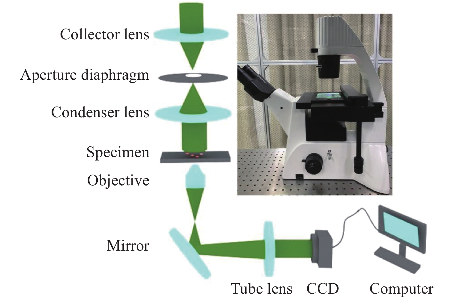
In this section, real experiments are carried out on samples of continuous distribution and discrete distribution respectively. A small amount of intensity images are collected by inverted microscope (MI52, Mshot), and the acquisition interval of adjacent intensity images is 2 μm. The experimental device and internal optical path are shown in Fig.7. The illumination light source is the LED white light in the microscope. Firstly, it passes through a optical filter with a center wavelength of 532 nm and half-peak bandwidth of 22 nm. Then the light intensity adjusted by a light collector and an aperture diaphragm. Next, we obtain uniform collimated light through a light collector. The light irradiates the sample through the objective lens, the reflector and the lens barrel lens. Finally, the enlarged object light field is transmited to the camera port of the microscope. The resolution of CCD (MS60, Mshot) used in the experiment is 2048×2048 pixel.

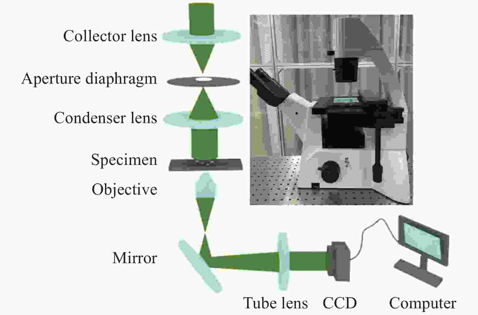
Figure 7.  Experimental device diagram and internal optical path

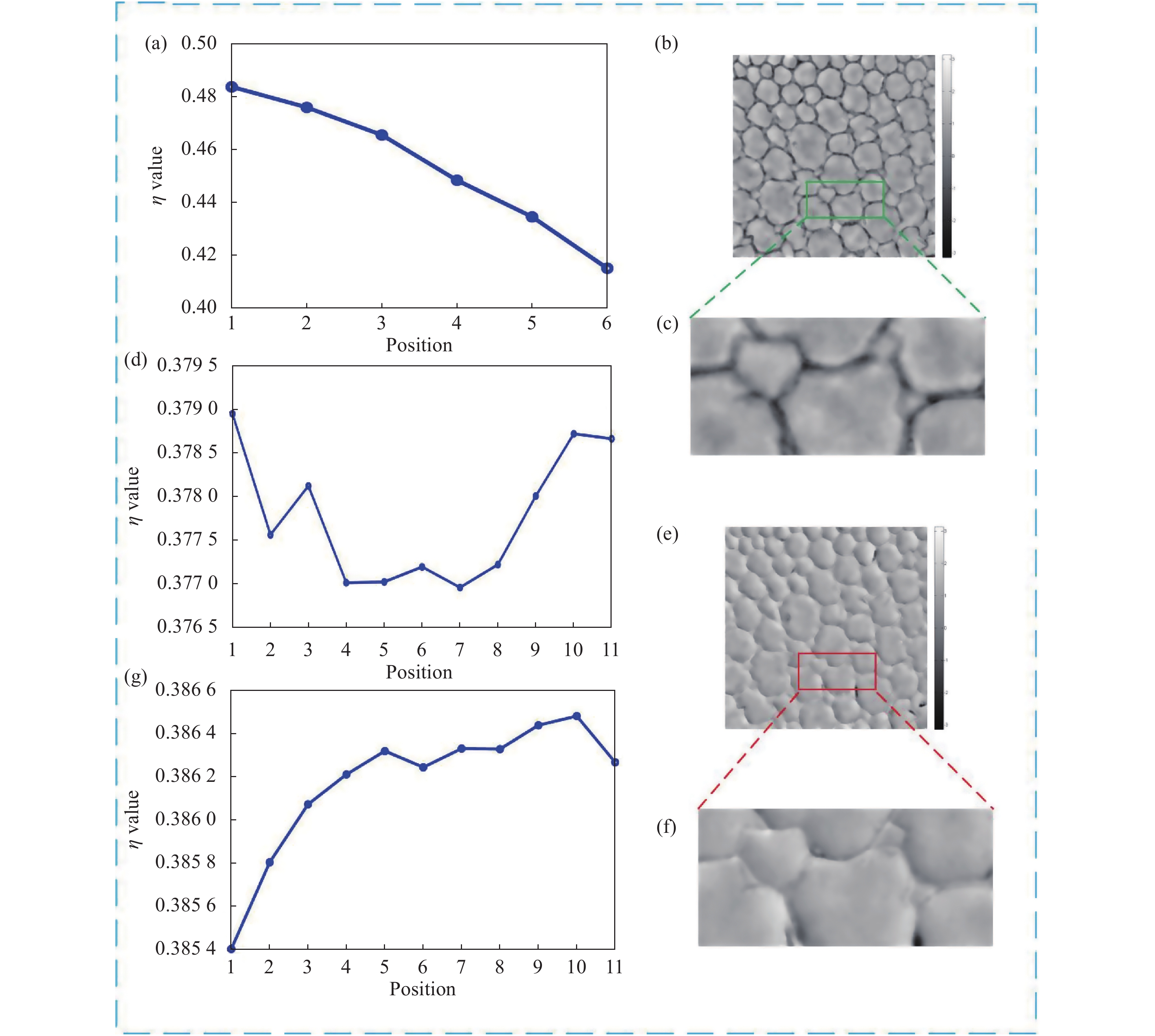
The continuous distributed cross-cutting cells of plant rhizomes are selected as sample in the real experiment of continuous distributed samples. EDR-TIE algorithm is used to locate the collected intensity images. The results are shown in Fig.8(a), and the positioning results are ideally located at the head or tail of a series of images. The phase is solved by using the intensity image and the corresponding defocus images of EDR-TIE positioning position, as shown in Fig.8(b). 10 intensity images are obtained from the EDR-TIE positioning position through angle spectrum propagated, since a new series of intensity images are obtained. Then AF-TIE calculation and edge duty ratio positioning are carried out. The positioning position is shown in Fig.8(d). Move the translation table to the AF-TIE positioning position to obtain the corresponding intensity images, then solve the phase, as shown in Fig.8(e). Once again, 10 intensity images are obtained through forward angle spectrum propagation, and edge duty ratio positioning is carried out. As shown in Fig.8(g). It is found that the located position has not changed. So the cycle can be ended.

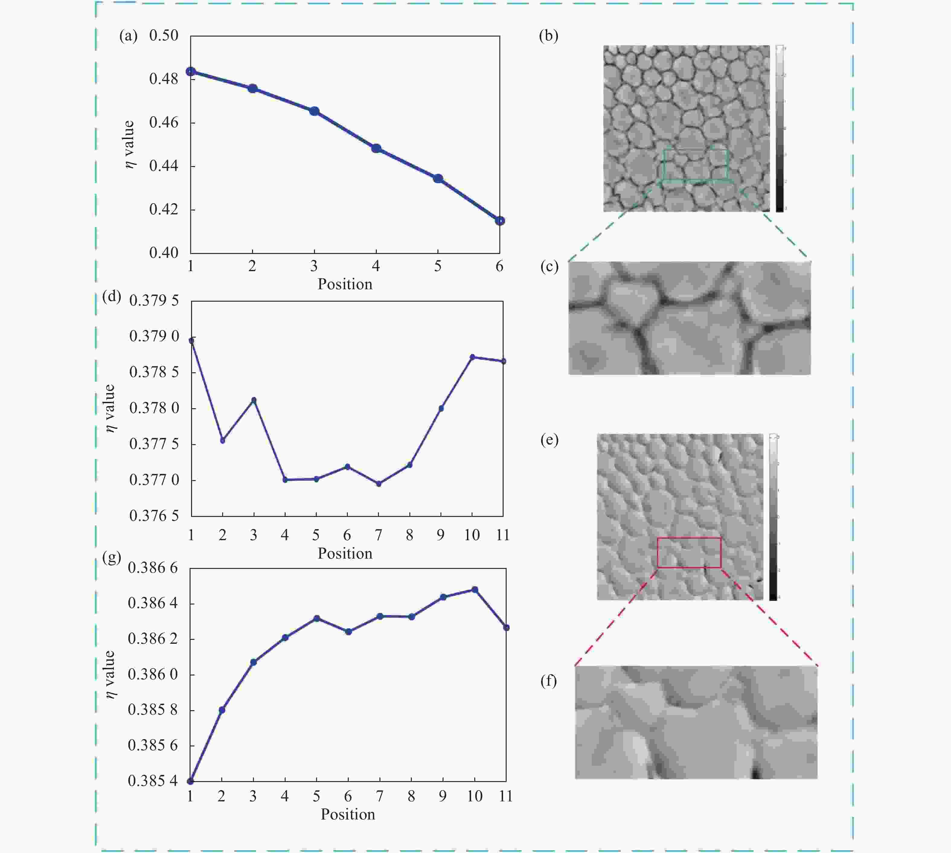
Figure 8.  Real experiment-plant rhizome cross section. (a) EDR-TIE positioning calculation result diagram; (b) EDR-TIE positioning position phase result diagram; (c) Partially enlarged phase result diagram of (b); (d) AF-TIE positioning calculation result diagram; (e) AF-TIE positioning position phase result diagram; (f) Partially enlarged phase result diagram of (e); (g) Optimal focus position angle spectrum AF-TIE positioning calculation result diagram

Figure8(c) and Figure8(f) are local amplification images of the phase results of Figure8(b) and Figure8(e) respectively. It can be seen that the optimal focus position can be located through several cycles by using AF-TIE algorithm.

In order to quantitatively evaluate the clarity of the retrieval phase, we use the edge duty ratio to compare the retrieval phase of EDR-TIE algorithm with AF-TIE algorithm, and the results are shown in Tab.2. It can be seen from the comparison result that when the initial image sequence does not contain focus image, the edge duty ratio of retrieval phase of the AF-TIE positioning position is smaller than the EDR-TIE positioning position, that is, AF-TIE algorithm has higher accuracy than EDR-TIE algorithm.

In order to further prove that the focus position located by AF-TIE algorithm is the optimal focus position. We move the translation stage of the microscope to the position of 7, which is the focus position located by AF-TIE algorithm, then taking 3 images at the same distance before and after the 7 position (the interval is 2 μm) and directly using the edge duty ratio to locate the the optimal focus image of the 7 images. The 7 images and the positioning results are shown in Fig.9(a) and Fig.9(b). It can be seen from the results that the real shot images are also located at position 7. That is, the positioning result of the edge duty ratio on the real shot image is consistent with the positioning result of AF-TIE, which proves the accuracy of the algorithm in this paper.

Figure 9.  Validation of focused results. (a) 7 intensity images taken by the microscope; (b) Positioning result by edge duty ratio

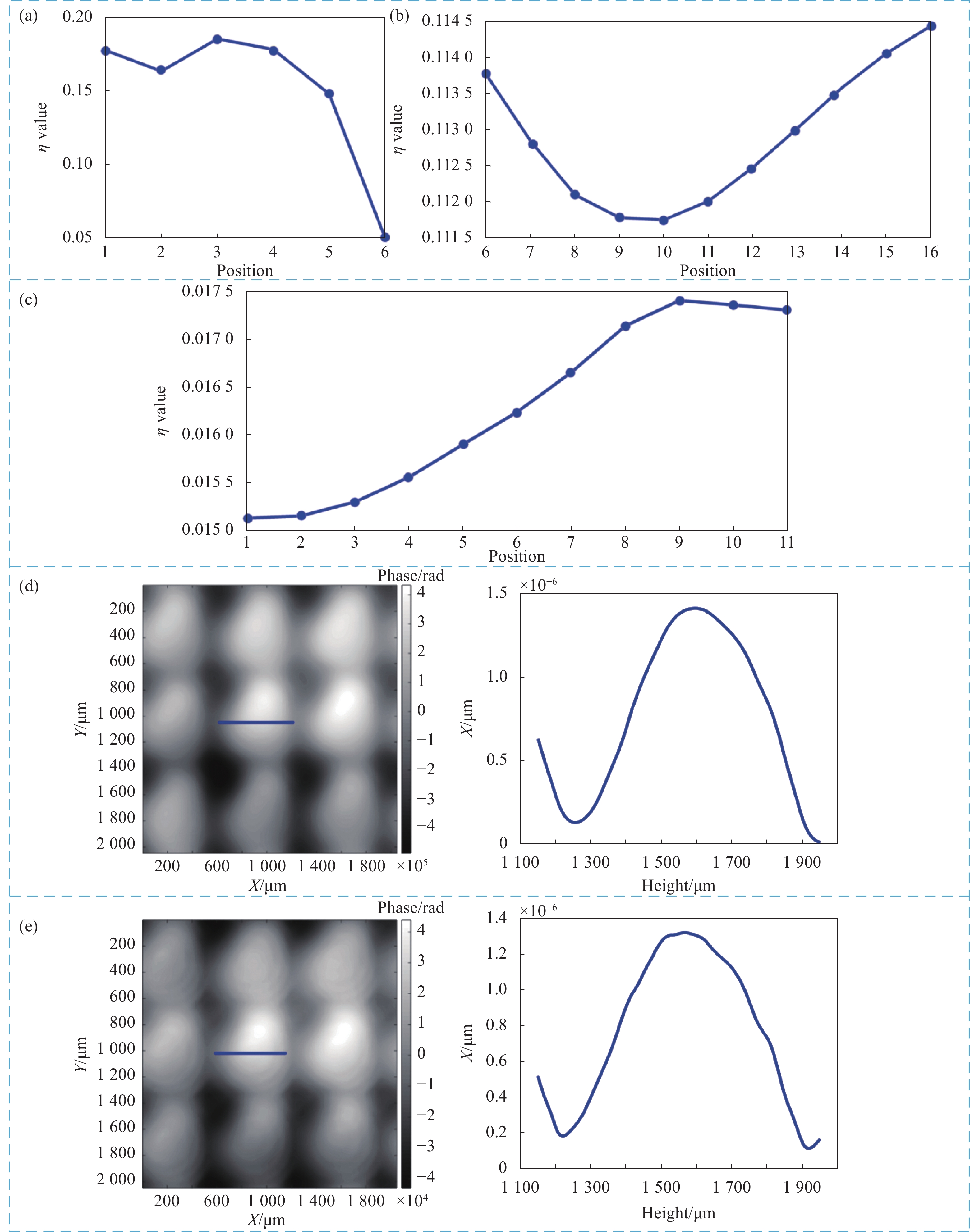
In this experiment, microlense (Thorlab) was choosed as sample, and the lens material was fused Shi Ying with refractive index of 1.458. EDR-TIE positioning results are shown in Fig.10(a), then solve the corresponding phase and cycle. The best focus positioning results in this paper are shown in Fig.10(b). Move the translation table to the best positioning position and capture the corresponding intensity image, then solve the phase. The phase results of the best positioning positions of EDR-TIE and AF-TIE are shown in the Fig.10(c) and Fig.10(d) respectively. The true height of the microlens array is 1.11 μm. The height of the microlens array at EDR-TIE position is 1.2805 μm with error of 15.3%. The height of the microlens array at optimal focusing position of AF-TIE is 1.1739 μm with error of 5.7%. The results show that the optimal focal plane phase height obtained by AF-TIE algorithm in this paper is closer to the real value.

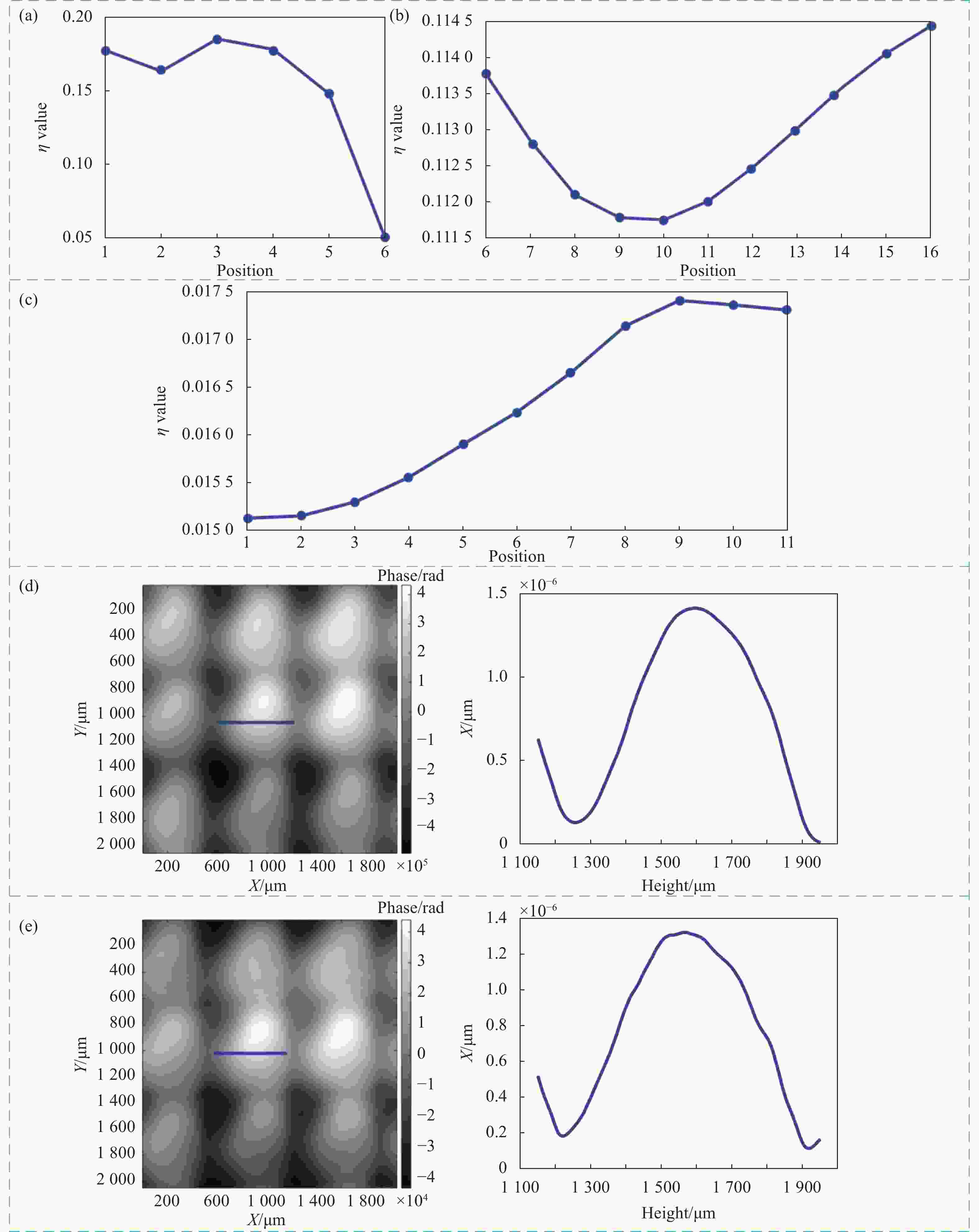
Figure 10.  Actual experience micro lens array: (a) EDR-TIE positioning results; (b) AF-TIE was the best position result; (c) The optimal focus position angular spectrum AF-TIE positioning calculation result; (d) EDR-TIE position phase result and solid line section height curve; (e) AF-TIE position phase results and solid line section height curve

In the solving process of TIE, the focus image is needed to participate. The accurate positioning of focused image is vital to improve the accuracy of phase retrieval. In the field of microscopic imaging, AF-TIE algorithm can be used to locate the optimal focus position. For a series of images collected by microscope. Firstly, solve the phase of the first positioning position which located by the egde duty ratio. Then the circular angular spectrum propagation and focus judgment is carried out until the lacation postion remains unchanged. Where it is finally located is the optimal focus position. The AF-TIE algorithm reduce the time to obtain a large number of images, which promotes to the development of automatic focusing technology and improves the accuracy of phase retrieval.