


-
图像在人类的生产生活中扮演着获取信息和传递信息的重要角色。随着成像技术的发展,图像的获取来源越来越丰富。在很多时候,往往需要对同一场景使用多种探测器联合成像,以满足不同的应用需求。例如,在成像探测领域,红外传感器通过获取场景中物体的热辐射信息进行成像,因此红外图像对热辐射明显的物体更为敏感,但这是以损失了空间分辨率为代价的,红外图像的空间分辨率低、纹理特征模糊;而可见光探测器虽然具有很高的空间分辨率,但是其原理是接收场景的反射光线进行成像,因此非常依赖于光线的强弱,一旦光强很弱、被遮挡或者目标采用了光学隐身伪装,那么可见光成像将难以发现场景中的目标。在这种情况下,往往需要同时利用红外图像和可见光图像中的互补信息,才能采集场景中完整的信息,这势必给场景采集带来了更多复杂度[1]。
文中主要应用于红外与可见光图像融合领域。当对同一场景进行红外成像与可见光成像时,可以获取两种传感器的信息,但同时也产生了冗余信息。红外探测器对场景中物体的热辐射较为敏感,所以在光照条件不足时依然可以工作。而可见光探测器对可见光波段的信息更加敏感,其图像拥有更清晰的纹理和更高的分辨率。因此,若能将红外探测器与可见光探测器所成的图像结合起来得到一幅复合图像,可以更加完整的描述场景信息,观察者也能更好的理解场景信息,从而做出进一步可能的决策。此外,还能去除大部分的冗余信息,节省存储空间[2]。
-
近年来,红外图像与可见光图像融合技术发展迅速,其中应用最为广泛的一种方法是多尺度变换(MST)方法[3]。MST方法的基本步骤是先将源图像分解为低频子带与高频子带,再使用不同的融合策略对不同的子带进行融合,最后利用相应的MST逆变换将融合图像重构出来。传统的MST方法包括小波变换方法,轮廓波变换方法,以及剪切波变换方法。由于MST方法可以在不同尺度对源图像进行融合,因而从大尺度结构到小尺度细节均被有效利用。但由于进行具体某一多尺度变换的基本函数都是固定的,所以一旦源图像没有完美配准,那么融合图像在局部图像块中会损失信息。
另一类融合方法称为梯度变换融合(GTF)方法[4]。该方法提出了一个总体变异模型,利用该模型能够同时保留红外图像中目标的分布和可见光图像的梯度变换。但是,并没有使用到可见光图像的强度信息,这可能导致图像的灰度值范围过于狭窄,并因此而丢失很多细节信息。
除了以上方法,边缘保持滤波(EPF)[5-6]也成功应用在了图像融合领域。EPF最大的优点是其在平滑图像的同时,可以最大程度的减小边缘信息的损失。由于EPF具有如此优越的特性,它能够被应用到很多领域。近年来,EPF在图像融合领域的应用也非常多,典型的基于EPF的图像融合方法包括双边滤波(BF)方法[7]和引导图像滤波(GIF)方法[8]。但EPF方法的融合结果在平滑时,纹理细节被平滑的也较多,因而融合结果容易会产生局部拼凑痕迹。
此后,Zhou等人[9]提出了一种非常有效的融合方法,将其称为混合多尺度分解感知融合(HMSD)方法。该HMSD方法利用了多次的高斯滤波与双边滤波(BF)后的结果进行交替差分,得到了源图像的细尺度边缘特征与粗尺度边缘特征,不同尺度的边缘特征采用不同的融合规则,最终的融合结果便于人类或机器进行感知。但该方法使用的双边滤波未能充分考虑低对比度信息,低对比度信息在双边滤波时也被同时滤掉,造成融合图像可能出现看起来不自然的视觉效果。为了克服这个缺点,Zhou等人[10]之后对其进行了改进,将模型中的BF替换为GIF,并将高斯滤波移除,该方法称为改进的HMSD (IHMSD)融合方法。IHMSD方法在红外图像与低光照条件下的可见光图像融合时效果非常理想,但是由于GIF本身的自由参数较多,所以调参过程复杂,且当场景变换时,需要重新进行调参;同时IHMSD方法在红外图像与正常光照条件下的可见光图像融合时效果并没有显著提升。不过,虽然HMSD模型存在上述缺陷,但它无疑提供了利用EPF进行图像分解的重要思路。受HMSD图像分解模型的启发,文中提出的算法也利用了HMSD图像分解模型的大框架,不同点为将HMSD框架中的双边滤波以及IHMSD框架中的引导滤波替换为了加权平均曲率滤波。
与前人提出的算法相比,文中提出的算法具有以下创新点:
(1)文中提出了一种基于加权平均曲率滤波与高斯滤波交替差分相结合的图像分解模型,能够将源图像分解为三种不同尺度的层级。
(2)源图像被分解为3种不同尺度的层级之后,每个层级根据其表征的图像特性不同,采用了3种不同的融合策略进行融合。
-
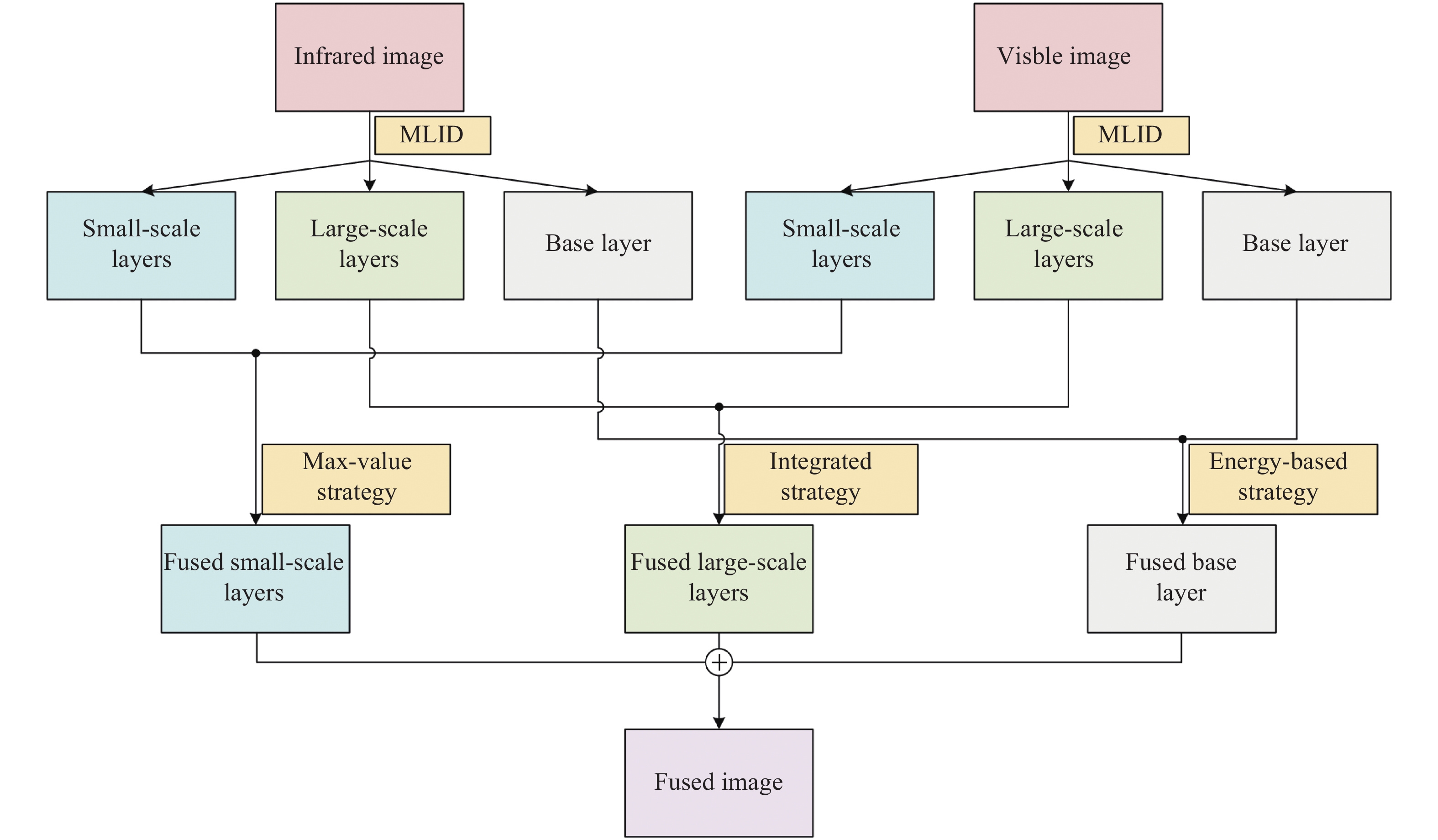
文中提出的图像融合算法的流程图如图1所示,具体步骤为:首先,利用加权平均曲率滤波的边缘保持特性与高斯滤波的平滑特性,构建多层级图像分解模型(MLID);再利用该模型将源图像分解为小尺度层、大尺度层和基层等3个不同层级;然后,针对基层,采用能量属性融合策略进行融合;针对大尺度层,采用复合融合策略进行融合;针对小尺度层,采用最大值融合策略;最后,将融合后的层级进行加和,以重构出最终的融合图像。

图 1 文中算法流程图
Figure 1. Flowchart of the proposed algorithm
-
对于一幅图像U而言,其加权平均曲率滤波定义为:
$$ {H^w}\left( U \right) = n{\left\| {\nabla U} \right\|_2}\left( {\nabla \cdot \frac{{\nabla U}}{{{{\left\| {\nabla U} \right\|}_2}}}} \right) $$ (1) 式中:
$ \nabla $ 和$ \nabla \cdot $ 分别表示梯度运算和散度运算符号。对二维图形而言,n = 2,则公式(1)可变化为:
$$ {H^w}\left( U \right) = \Delta U - \frac{{U_y^2{U_{yy}} + 2{U_x}{U_y}{U_{xy}} + U_x^2{U_{xx}}}}{{U_x^2 + U_y^2}} $$ (2) 式中:∆表示各向同性的拉普拉斯算子;Ux和Uy表示U在x和y方向上的一阶偏微分;Uxx、Uyy和Uxy表示相应的二阶偏微分。公式(2)的具体推导方法可参考文献[11],这里不再赘述。
公式(2)是加权平均曲率滤波的连续形势的定义,而实际图像都是离散的像素点,因此需要定义离散形势的加权平均曲率滤波。
对于一个3×3大小的窗口,存在8种可能的归一化半窗口方向,这8种情况分别服从下列核矩阵:
$$ \begin{split}& {h_1} = \left[ {\begin{array}{*{20}{c}} {1/6}&{1/6}&0 \\ {1/3}&{ - 1}&0 \\ {1/6}&{1/6}&0 \end{array}} \right]{\text{ }}{h_2} = \left[ {\begin{array}{*{20}{c}} {1/6}&{1/3}&{1/6} \\ {1/6}&{ - 1}&{1/6} \\ 0&0&0 \end{array}} \right] \\& {h_3} = \left[ {\begin{array}{*{20}{c}} 0&{1/6}&{1/6} \\ 0&{ - 1}&{1/3} \\ 0&{1/6}&{1/6} \end{array}} \right]{\text{ }}{h_4} = \left[ {\begin{array}{*{20}{c}} 0&0&0 \\ {1/6}&{ - 1}&{1/6} \\ {1/6}&{1/3}&{1/6} \end{array}} \right] \\& {h_5} = \left[ {\begin{array}{*{20}{c}} {1/6}&{1/3}&{1/12} \\ {1/3}&{ - 1}&0 \\ {1/12}&0&0 \end{array}} \right]{\text{ }}{h_6} = \left[ {\begin{array}{*{20}{c}} {1/12}&{1/3}&{1/6} \\ 0&{ - 1}&{1/3} \\ 0&0&{1/12} \end{array}} \right] \\& {h_7} = \left[ {\begin{array}{*{20}{c}} 0&0&{1/12} \\ 0&{ - 1}&{1/3} \\ {1/12}&{1/3}&{1/6} \end{array}} \right]{\text{ }}{h_8} = \left[ {\begin{array}{*{20}{c}} {1/12}&0&0 \\ {1/3}&{ - 1}&0 \\ {1/6}&{1/3}&{1/12} \end{array}} \right] \end{split} $$ (3) 根据公式(3)的8个核函数可以计算出8个距离
$$ {d_k} = {h_k}*U,k = 1,2, \cdots ,8 $$ (4) 式中:*表示卷积运算符号。则公式(2)的离散形势可表示为:
$$ {H^w} = {d_m},{\text{ }}m = {\text{argmin}}\left| {{d_k}} \right| $$ (5) 为方便起见,文中使用下式表示加权平均曲率滤波运算:
$$ {I_f} = WMC\left( {{I_{in}}} \right) $$ (6) 式中:Iin和If分别是输入图像和滤波后的图像;WMC(•)表示加权平均曲率滤波运算函数。
-
高斯滤波(GF)是一种能够用于图像降质和图像平滑的非常经典的工具,通过高斯滤波操作能够获得大部分的图像低频信息。文中提出的多层级图像分解模型充分利用了加权平均曲率滤波与高斯滤波的特性,通过多层级图像分解模型,能够得到图像的各尺度层的信息。多层级图像分解模型的算法结构图如图2所示。

图 2 多层级图像分解模型流程图
Figure 2. Flowchart of the multi-level image decomposition model
图中,Iin代表输入图像,
$ I_g^{\left( i \right)} $ 表示第i次高斯滤波的结果,$ I_f^{\left( i \right)} $ 表示第i次加权平均曲率滤波的结果,B是基层,FS(i)和CS(i)分别表示第i层的粗略特征子图和细微特征子图,3种层的计算公式分别为:$$ F{S^{\left( i \right)}} = \left\{ {\begin{array}{*{20}{l}} {{I_{in}} - I_f^{\left( i \right)},i = 1{\text{ }}} \\ {I_g^{\left( {i - 1} \right)} - I_f^{\left( i \right)},i = 2,3} \end{array}} \right. $$ (7) $$ C{S^{\left( i \right)}} = I_f^{\left( i \right)} - I_g^{\left( i \right)} $$ (8) $$ BS = I_g^{\left( 3 \right)} $$ (9) 其中,
$ I_g^{\left( i \right)} $ 和$ I_f^{\left( i \right)} $ 分别表示为:$$ I_g^{\left( i \right)} = \left\{ {\begin{array}{*{20}{l}} {GF\left( {{I_{in}}} \right),i = 1{\text{ }}} \\ {GF\left( {I_g^{\left( {i - 1} \right)}} \right),i = 2,3} \end{array}} \right. $$ (10) $$ I_f^{\left( i \right)} = \left\{ {\begin{array}{*{20}{l}} {WMC\left( {{I_{in}}} \right),i = 1{\text{ }}} \\ {WMC\left( {I_g^{\left( {i - 1} \right)}} \right),i = 2,3} \end{array}} \right. $$ (11) 式中:GF(·)表示高斯滤波算子。
-
红外图像包含强边缘和结构特征,而可见光图像包含更多空间细节信息。由于他们表征的信息不一致,如果采用与传统多尺度变换方法类似的操作进行像素融合,那么融合图像中很可能含有视觉上看起来“不正常”的区域。因此,在像素融合前,需要提取两类源图像不同层的主要特征。红外与可见光图像融合的本质是将红外图像中的显著性特征信息注入到可见光图像中,所以要保证红外图像的显著特征被正确的探测到。分解出的层在不同尺度下具有不同的特征,因此各个尺度的融合需要采用不同的融合策略。
为方便表示,文中使用IIR和IVis代表输入的红外图像与可见光图像,
$ FS_{IR}^{\left( i \right)} $ 、$ FS_{Vis}^{\left( i \right)} $ 、$ CS_{IR}^{\left( i \right)} $ 、$ CS_{Vis}^{\left( i \right)} $ 、BIR、BVis分别表示红外图像和可见光图像的粗略特征子图、细微特征子图和基层子图。 -
源图像中的纹理特征信息主要在小尺度层中,这些信息若能尽可能多的保留在融合图像中,则能够提升融合图像的质量。对于红外图像而言,像素值越大的部分,表明目标越突出,其更应该保留在融合图像中。因此,在小尺度层中采取最大值融合策略,融合的小尺度层可以表示为:
$$ Fu{F_1}\left( {x,y} \right) = {\text{max}}\left( {FS_{IR}^{\left( 1 \right)}\left( {x,y} \right),FS_{Vis}^{\left( 1 \right)}\left( {x,y} \right)} \right) $$ (12) $$ Fu{C_1}\left( {x,y} \right) = {\text{max}}\left( {CS_{IR}^{\left( 1 \right)}\left( {x,y} \right),CS_{Vis}^{\left( 1 \right)}\left( {x,y} \right)} \right) $$ (13) 式中:(x, y)表示像素的坐标。
-
源图像中的边缘及结构信息都包含在大尺度层中,为了将红外图像的边缘和结构注入到可见光图像中,对大尺度层中的边缘特征和结构特征进行提取是很有必要的。文中提出一种复合融合策略,利用了图像的空间频率和局部方差。
(1)空间频率
图像的空间频率反映了图像的整体活跃度,对图像I中大小为P×Q的一块区域,其行频率(RF)与列频率(CF)分别定义为:
$$ RF = \sqrt {\frac{1}{{PQ}}\sum\limits_{x = 1}^P {{{\sum\limits_{y = 2}^Q {\left[ {I\left( {x,y} \right) - I\left( {x,y - 1} \right)} \right]} }^2}} } $$ (14) $$ CF = \sqrt {\frac{1}{{PQ}}\sum\limits_{y = 1}^Q {{{\sum\limits_{x = 2}^P {\left[ {I\left( {x,y} \right) - I\left( {x - 1,y} \right)} \right]} }^2}} } $$ (15) 则空间频率(SF)定义为:
$$ S F = \sqrt {RF{{\left( {x,y} \right)}^2} + CF{{\left( {x,y} \right)}^2}} $$ (16) (2)局部方差
图像的局部方差衡量了局部图像清晰度和对比度,对于图像I中P×Q大小的图像块,其局部方差(LV)计算公式为:
$$ S F = \sum\limits_{r = - P/2}^{P/2} {\sum\limits_{s = - Q/2}^{Q/2} {\frac{{{{\left[ {I\left( {x + r,y + s} \right) - \mu } \right]}^2}}}{{P \times Q}}} } $$ (17) 式中:μ表示I中该图像块中所有像素的平均值。
(3)复合融合策略
大尺度层分别用
$ FS_{IR}^{\left( i \right)} $ 、$ FS_{Vis}^{\left( i \right)} $ 、$ CS_{IR}^{\left( i \right)} $ 、$ CS_{Vis}^{\left( i \right)} $ 表示,每个量的空间频率与局部方差具体可见表1。表 1 四种大尺度层的空间频率及局部方差
Table 1. Four types large-scale layers and their spatial frequency and local variance
Measures SF LV $ FS_{IR}^{\left( i \right)} $ $ SF_{FIR}^{\left( i \right)} $ $ LV_{FIR}^{\left( i \right)} $ $ FS_{Vis}^{\left( i \right)} $ $ SF_{FVis}^{\left( i \right)} $ $ LV_{FVis}^{\left( i \right)} $ $ CS_{IR}^{\left( i \right)} $ $ SF_{CIR}^{\left( i \right)} $ $ LV_{CIR}^{\left( i \right)} $ $ CS_{Vis}^{\left( i \right)} $ $ SF_{CVis}^{\left( i \right)} $ $ LV_{CVis}^{\left( i \right)} $ 复合融合策略采用空间频率与局部方差获取的大尺度层FuFi和FuCi (i = 2,3),其具体计算公式为:
$$ Fu{F}_{i}\left(x,y\right)=\Bigg\{\begin{array}{l}F{S}_{IR}^{\left(i\right)},若S {F}_{FIR}^{\left(i\right)} > S{F}_{FVis}^{\left(i\right)}且L{V}_{FIR}^{\left(i\right)} > L{V}_{FVis}^{\left(i\right)}\\ F{S}_{Vis}^{\left(i\right)},其他情况\end{array} $$ (18) $$ Fu{C}_{i}\left(x,y\right)=\Bigg\{\begin{array}{l}C{S}_{IR}^{\left(i\right)},若S {F}_{CIR}^{\left(i\right)} > S{F}_{CVis}^{\left(i\right)}且L{V}_{CIR}^{\left(i\right)} > L{V}_{CVis}^{\left(i\right)}\\ C{S}_{Vis}^{\left(i\right)},其他情况\end{array} $$ (19) -
背景中的大多数信息以及最粗略的结构都集中在源图像的基层中,因此基层的融合对融合图像的整体质量起到了决定性作用。由于基层包含了源图像的大多数信息,因此使用基于自然指数的能量属性融合策略,该融合策略主要分为3个步骤:
Step1:计算基层的本征属性,分别用SIR和SVis表示:
$$ \left\{ {\begin{array}{*{20}{l}} {{S_{IR}} = {\mu _{IR}} + {M_{IR}}} \\ {{S_{Vis}} = {\mu _{Vis}} + {M_{Vis}}} \end{array}} \right. $$ (20) 式中:μIR、μVis、MIR、MVis分别代表红外与可见光图像的基层的均值和中值。 Step2:计算基层的能量属性函数,分别用EIR与EVis表示:
$$ \left\{ {\begin{array}{*{20}{l}} {{E_{IR}}\left( {x,y} \right) = {\text{exp}}\left( {\alpha \left| {{B_{IR}}\left( {x,y} \right) - {S_{IR}}} \right|} \right)} \\ {{E_{Vis}}\left( {x,y} \right) = {\text{exp}}\left( {\alpha \left| {{B_{Vis}}\left( {x,y} \right) - {S_{Vis}}} \right|} \right)} \end{array}} \right. $$ (21) 式中:exp(•)表示自然指数函数;α表示增益系数。
Step3:通过加权融合方法计算得到融合后的基层:
$$ FuB\left( {x,y} \right) = \frac{{{E_{IR}}\left( {x,y} \right) \cdot {B_{IR}}\left( {x,y} \right) + {E_{Vis}}\left( {x,y} \right) \cdot {B_{Vis}}\left( {x,y} \right)}}{{{E_{IR}}\left( {x,y} \right) + {E_{Vis}}\left( {x,y} \right)}} $$ (22) -
融合图像FuI可以通过融合后的3种层进行加和重构,具体表达式为:
$$ FuI = \sum\limits_{i = 1}^3 {\left( {Fu{F_i} + Fu{C_i}} \right) + FuB} $$ (23) -
文中提出的算法将会与现有的几种优秀的融合算法进行定性比较与定量比较,这些算法包括均非下采样轮廓波方法(NSCT)[3]、引导图像滤波方法(GIF)[8]、梯度变换方法(GTF)[4]、混合多尺度分解方法(HMSD)[9]、改进的混合多尺度分解方法(IHMSD)[10]。
-
红外与可见光图像融合的目的是获得一幅具有更高空间分辨率,且更有利于识别目标的复合图像,文中采用了进行了三组实验,各组实验的源图像以及几种算法的融合结果如图3~图5所示。其中各组图的图(a)和(b)分别为红外图像与可见光图像,图(c)~(h)分别为NSCT方法、GIF方法、GTF方法、HMSD方法、IHMSD方法以及文中算法,各个对比算法的缺陷在图中以用红色矩形框标识出来。

图 3 第一组实验的各方法对比结果
Figure 3. Comparison results of each method of the first set of experiments

图 4 第二组实验的各方法对比结果
Figure 4. Comparison results of each method of the second set of experiments

图 5 第三组实验的各方法对比结果
Figure 5. Comparison results of each method of the third set of experiments
在第一组实验中,NSCT方法的融合结果较差,图3(c)中人与背景的对比度较低,篱笆也几乎难以被看到;GIF方法的融合结果相对较好,但图3(d)中的篱笆也难以被看到,下方的植物也没有继承相对清晰的可见光图像的背景;GTF方法的融合结果最差,图3(e)中人与背景的对比度最低,下方的植物几乎继承了红外图像中背景的模糊一片;图3(f)中的篱笆难以被分辨,植物没有继承可见光中清晰的背景;图3(g)的效果整体较好,但红框中建筑物的棱角过渡不自然;而文中提出的算法不存在上述问题,从图3(h)可以看出,人与背景的对比度较高,且背景中的物体大多较为清晰,有利于识别出复杂场景中隐藏于背景中的人。
在第二组实验中,NSCT方法的融合结果不理想,图4(c)中人和门的亮度不够,细节方面更接近于红外图像;GIF方法的融合结果略微好一些,但图4(d)上方的天空中出现了像素突变现象;GTF方法的融合结果最差,图4(e)虽然继承了红外图像中清晰的人体轮廓,但天空也继承了红外图像中漆黑一片的天空;图4(f)与图4(g)的整体效果较好,除了右上角均存在像素突变现象;而文中提出的算法不存在上述问题,从图4(h)可以看出,在尽可能保留更多可见光图像细节的同时,也能突显隐藏在背景中的人的对比度,非常有利于目标识别。
在第三组实验中,NSCT方法的融合结果灰度值降低比较明显,且图像变的比可见光图像模糊;GIF方法的融合结果的天空与地面都较为模糊,丢失了可见光图像中的细节信息;GTF方法的融合结果依旧效果最差,从可见光图像中继承的背景较少,图像整体较模糊;IHMSD方法的融合结果在左下方地面处的纹理不太清晰;HMSD方法的融合结果与文中提出的算法的融合结果不存在上述问题,融合的视觉效果相对较好,车身底部温度更高的部分较为明显,有利于进行目标识别。
-
视觉上的定性比较可以较为直观的评判融合结果的好坏,但这非常依赖于观察者自身的评判标准,不同的观察者对于同一幅图像可能有不同的评价结果,甚至同一观察者的心理状态都会影响融合的评价结果。因此客观的定量比较也是必不可少的。
文中采用信息熵(EN)[12]、结构相似度(SSIM)[13]、互信息(MI)[14]、整体融合指数(QT)[15]以及图像信息保真度(VIF)[16]等五种客观评价标准对融合结果进行比较。上述五种评价标准均是数值越大代表融合效果越好。
表2~表4给出了三组实验定量比较的结果,每一项标准的各算法的结果对应表格中的每一行,每一行结果的最大值用加粗字体表示。
表 2 第一组实验定量比较结果
Table 2. Quantitative comparison results of the first group of experiment
NSCT GIF GTF HMSD IHMSD Proposed EN 6.2409 6.3778 6.6779 6.6001 6.715 8 6.6007 SSIM 0.9989 0.9992 0.9991 0.9991 0.9991 0.9992 MI 1.6053 1.5275 2.0508 1.7595 1.7846 1.7883 QT 0.3623 0.4371 0.4358 0.4467 0.4520 0.4538 VIF 0.3199 0.2834 0.2185 0.4403 0.4319 0.4404 表 3 第二组实验定量比较结果
Table 3. Quantitative comparison results of the second group of experiment
NSCT GIF GTF HMSD IHMSD Proposed EN 6.5306 6.8575 6.9582 6.9566 6.9594 6.9643 SSIM 0.9990 0.9990 0.9991 0.9991 0.9992 0.9992 MI 2.1427 2.4550 2.5011 2.2770 2.2813 2.2845 QT 0.3323 0.4514 0.3145 0.4437 0.4472 0.4301 VIF 0.2966 0.2801 0.1843 0.3465 0.4350 0.3487 表 4 第三组实验定量比较结果
Table 4. Quantitative comparison results of the third group of experiment
NSCT GIF GTF HMSD IHMSD Proposed EN 6.4850 7.0175 7.0766 7.1275 7.1333 7.2041 SSIM 0.9985 0.9988 0.9988 0.9985 0.9988 0.9989 MI 1.8187 2.8373 2.0651 2.8486 2.8973 2.2845 QT 0.3357 0.4521 0.3360 0.4103 0.4206 0.4301 VIF 0.2704 0.1087 0.3276 0.3849 0.3943 0.3487 可以看到,第一组实验除了EN与MI这两项标准,文中提出的算法在其他三项标准均已达到最好的融合效果;第二组实验在EN与SSIM两项标准上,文中提出的算法达到了最好的融合效果;第三组实验与第二组一样,在EN与SSIM两项标准上,文中提出的算法达到了最好的融合效果。而IHMSD在其他的多数标准上也达到了最好的融合效果,从总体来看,文中提出的算法与IHMSD方法效果相当,在不同的标准上拥有各自的优势,但均没有在全部的情况下比对方的效果更好。鉴于IHMSD方法是近几年提出的一种处在世界领先水平的融合方法,而文中提出的算法能够与之旗鼓相当,所以文中提出的算法也是一种较为优秀的融合方法。
-
算法耗时是另一项重要的评价标准,运行速度快的算法有更好的实时性,也更有利于算法实际应用的落地。各算法运行消耗的时间如表5所示,可以看到,文中所提出的算法运行所消耗的时间与其他算法相比处在中间水平,还存在优化的空间。
表 5 各融合方法算法耗时(单位:秒)
Table 5. Time consumption of different fusion algorithm (Unit: s)
NSCT GIF GTF HMSD IHMSD Proposed First set 5.365 0.368 2.130 20.322 16.544 8.524 Second set 14.226 1.303 6.852 48.094 37.212 19.685 Third set 14.062 1.205 9.821 49.020 43.395 21.397 -
文中提出了一种基于多层级图像分解的红外与可见光图像融合算法。首先,利用加权平均曲率滤波的边缘保持特性与高斯滤波的平滑特性,构建了多层级图像分解模型。在利用该模型将源图像分解为小尺度层、大尺度层和基层等3个不同层级。然后,针对基层,采用能量属性融合策略进行融合;针对大尺度层,采用复合融合策略进行融合;针对小尺度层,采用最大值融合策略。最后,将融合后的层级进行加和,以重构出最终的融合图像。实验结果表明,文中提出算法的融合效果与处在世界领先水平的IHMSD方法效果相当,在不同的标准下有各自的优势,因此文中提出的算法也是一种较为优秀的融合方法。
需要注意的是,由于文中提出的算法在运行时间上还有待加强,未来研究的重点是优化算法,提高算法运行的效率,使其能够工程化。
Multi-layer image decomposition-based image fusion algorithm
-
摘要: 不同类型的探测器在成像机理上有不同的侧重点,使得成像图像表征的信息也有所不同,导致单幅图像不能完整地反映场景的有效信息。因此,提取多源图像的互补信息,并去除其中的冗余信息,合成一幅能准确、完整表达场景的复合图像的技术成为了图像处理领域中一项非常重要的技术,图像融合正是这类问题的一种有效解决方法。针对传统多尺度分解的图像融合方法易产生噪声和信息缺失的现象,文中提出了一种基于多层级图像分解的红外与可见光图像融合算法。首先,利用加权平均曲率滤波的边缘保持特性与高斯滤波的平滑特性,构建了多层级图像分解模型。在利用该模型将源图像分解为小尺度层、大尺度层和基层等3个不同层级。然后,针对基层,采用能量属性融合策略进行融合;针对大尺度层,采用复合融合策略进行融合;针对小尺度层,采用最大值融合策略。最后,将融合后的层级进行加和,以重构出最终的融合图像。实验结果表明:文中提出的基于多层级图像分解的图像融合算法能够有效降低噪声产生的概率,同时减少了融合后的信息缺失。Abstract: Different types of detectors have different imaging mechanisms, and the information represented by the image is also different in some ways, which results in the information of a scene cannot be completely descripted through a single image. Therefore, it is an important technology to extract complementary information of multi-source images, remove redundant information and synthesize a composite image which can express scene accurately and completely. Image fusion is an effective solution to this kind of problem. In this paper, an infrared and visible image fusion based on multi-layer image decomposition is proposed. Firstly, using the edge-preserving characteristics of weighted mean curvature filtering and the smoothing characteristics of Gaussian filtering, a multi-layer image decomposition model was constructed. Secondly, the source images were decomposed into small-scale layers, large-scale layers, and base layer. Thirdly, an energy attribute fusion strategy was adopted to merge the base layer, an integrated fusion strategy was adopted to merge the large-scale layers, and a max-value fusion strategy was adopted to merge the small-scale layers. Finally, the fused image was reconstructed through the sum operation of the three fused layers. Experimental results demonstrated that the proposed algorithm can effectively reduce the probability of noise generation and overcome the shortcomings of missing information in the fused image.
-
图 3 第一组实验的各方法对比结果
Figure 3. Comparison results of each method of the first set of experiments
图 4 第二组实验的各方法对比结果
Figure 4. Comparison results of each method of the second set of experiments
图 5 第三组实验的各方法对比结果
Figure 5. Comparison results of each method of the third set of experiments
表 1 四种大尺度层的空间频率及局部方差
Table 1. Four types large-scale layers and their spatial frequency and local variance
Measures SF LV $ FS_{IR}^{\left( i \right)} $ $ SF_{FIR}^{\left( i \right)} $ $ LV_{FIR}^{\left( i \right)} $ $ FS_{Vis}^{\left( i \right)} $ $ SF_{FVis}^{\left( i \right)} $ $ LV_{FVis}^{\left( i \right)} $ $ CS_{IR}^{\left( i \right)} $ $ SF_{CIR}^{\left( i \right)} $ $ LV_{CIR}^{\left( i \right)} $ $ CS_{Vis}^{\left( i \right)} $ $ SF_{CVis}^{\left( i \right)} $ $ LV_{CVis}^{\left( i \right)} $  下载: 导出CSV
表 2 第一组实验定量比较结果
Table 2. Quantitative comparison results of the first group of experiment
NSCT GIF GTF HMSD IHMSD Proposed EN 6.2409 6.3778 6.6779 6.6001 6.715 8 6.6007 SSIM 0.9989 0.9992 0.9991 0.9991 0.9991 0.9992 MI 1.6053 1.5275 2.0508 1.7595 1.7846 1.7883 QT 0.3623 0.4371 0.4358 0.4467 0.4520 0.4538 VIF 0.3199 0.2834 0.2185 0.4403 0.4319 0.4404
下载: 导出CSV
表 3 第二组实验定量比较结果
Table 3. Quantitative comparison results of the second group of experiment
NSCT GIF GTF HMSD IHMSD Proposed EN 6.5306 6.8575 6.9582 6.9566 6.9594 6.9643 SSIM 0.9990 0.9990 0.9991 0.9991 0.9992 0.9992 MI 2.1427 2.4550 2.5011 2.2770 2.2813 2.2845 QT 0.3323 0.4514 0.3145 0.4437 0.4472 0.4301 VIF 0.2966 0.2801 0.1843 0.3465 0.4350 0.3487
下载: 导出CSV
表 4 第三组实验定量比较结果
Table 4. Quantitative comparison results of the third group of experiment
NSCT GIF GTF HMSD IHMSD Proposed EN 6.4850 7.0175 7.0766 7.1275 7.1333 7.2041 SSIM 0.9985 0.9988 0.9988 0.9985 0.9988 0.9989 MI 1.8187 2.8373 2.0651 2.8486 2.8973 2.2845 QT 0.3357 0.4521 0.3360 0.4103 0.4206 0.4301 VIF 0.2704 0.1087 0.3276 0.3849 0.3943 0.3487
下载: 导出CSV
表 5 各融合方法算法耗时(单位:秒)
Table 5. Time consumption of different fusion algorithm (Unit: s)
NSCT GIF GTF HMSD IHMSD Proposed First set 5.365 0.368 2.130 20.322 16.544 8.524 Second set 14.226 1.303 6.852 48.094 37.212 19.685 Third set 14.062 1.205 9.821 49.020 43.395 21.397
下载: 导出CSV
-
[1] Dai Jindun, Liu Yadong, Mao Xianyin, et al. Infrared and visible image fusion based on FDST and dual-channel PCNN [J]. Infrared and Laser Engineering, 2019, 48(2): 0204001. (in Chinese) [2] Zeng Hanlin, Meng Xiangyong, Qian Weixian. Image fusion algorithm based on DOG filter [J]. Infrared and Laser Engineering, 2020, 49(S1): 20200091. (in Chinese) [3] Zhao Chunhui, Guo Yunting, Wang Yulei. A fast fusion scheme for infrared and visible light images in NSCT domain [J]. Infrared Physics & Technology, 2020, 72: 266-275. [4] Ma Jiayi, Chen Chen, Li Chang, et al. Infrared and visible image fusion via gradient transfer and total variation minimization [J]. Information Fusion, 2016, 31: 100-109. doi: 10.1016/j.inffus.2016.02.001 [5] Tan Wei, Xiang Pei, Zhang Jiajia, et al. Remote sensing image fusion via boundary measured dual-channel PCNN in multi-scale morphological gradient domain [J]. IEEE Access, 2020, 8: 42540-42549. doi: 10.1109/ACCESS.2020.2977299 [6] Tan Wei, Zhou Huixin, Song Jiangluqi, et al. Infrared and visible image perceptive fusion through multi-level Gaussian curvature filtering image decomposition [J]. Applied Optics, 2019, 58(12): 3064-3073. doi: 10.1364/AO.58.003064 [7] Hu Jianwen, Li Shutao. The multiscale directional bilateral filter and its application to multisensory image fusion [J]. Information Fusion, 2012, 13(3): 196-206. doi: 10.1016/j.inffus.2011.01.002 [8] Li Shutao, Kang Xudong, Hu Jianwen. Image fusion with guided filtering [J]. IEEE Transactions on Image Processing, 2013, 22(7): 2864-2875. doi: 10.1109/TIP.2013.2244222 [9] Zhou Zhiqiang, Wang Bo, Li Sun, et al. Perceptual fusion of infrared and visible images through a hybrid multi-scale decomposition with Gaussian and bilateral filters [J]. Information Fusion, 2016, 30: 15-26. doi: 10.1016/j.inffus.2015.11.003 [10] Zhou Zhiqiang, Dong Mingjie, Xie Xiaozhu, et al. Fusion of infrared and visible images for night-vision context enhancement [J]. Applied Optics, 2016, 55(23): 6480-6490. doi: 10.1364/AO.55.006480 [11] Gong Yuanhao, Goksel Orcun. Weighted mean curvature [J]. Signal Processing, 2019, 164: 329-339. doi: 10.1016/j.sigpro.2019.06.020 [12] Wesley R J, van Aardt Jan A, Babikker A F. Assessment of image fusion procedures using entropy, image quality, and multispectral classification [J]. Journal of Applied Remote Sensing, 2008, 2(1): 023522. doi: 10.1117/1.2945910 [13] Wang Zhou, Conrad B A, Rahim S H, et al. Image quality assessment: From error visibility to structural similarity [J]. IEEE Transactions on Image Processing, 2004, 13(4): 600-612. doi: 10.1109/TIP.2003.819861 [14] Qu Guihong, Zhang Dali, Yan Pingfan. Information measure for performance of image fusion [J]. Electronics Letters, 2002, 38(7): 313-315. doi: 10.1049/el:20020212 [15] Yu Xianchuan, Pei Wenjing. Performance evaluation of image fusion quality metrics for the quality of different fusion methods [J]. Infrared and Laser Engineering, 2012, 41(12): 3416-3422. (in Chinese) [16] Han Yu, Cai Yunze, Cao Yin, et al. A new image fusion performance metric based on visual information fidelity [J]. Information Fusion, 2013, 14(2): 127-135. doi: 10.1016/j.inffus.2011.08.002 -

 点击查看大图
计量
- 文章访问数: 269
- HTML全文浏览量: 55
- PDF下载量: 64
- 被引次数: 0


