


-
非本征光纤法珀传感(Extrinsic Fabry-Perot Interferometric, EFPI)是当下光纤传感器研究领域的一个重要分支,因为易于集成且不受电磁干扰等优点[1],在复合材料、大型建筑结构、军工产品等的结构健康自诊断、医疗微创器械位置追踪等领域都有广阔的应用前景[2]。随着传感技术的发展,在如超大规模集成电路制作、复杂环境下的探测等领域都需要更高精度的传感器[3],而对其光谱解调方法是决定其能否实现高精度测量的关键。
EFPI传感器腔长信号解调方法主要分为强度解调和相位解调。强度解调法原理简单且成本低[4],但光源自身稳定因素的影响对解调结果影响较大,精确度不高。三波长自适应强度解调法可以解决光源稳定问题[5],且测量范围大,但是解调速度慢。传统相位解调法有高灵敏度高分辨率等优点,但仍然不适合高速测量[6]。田培廷[7]提出将波长不同的2束呈正交光由单光纤经耦合器送入F-P腔,然后再通过密集波分复用器将两个波长的反射光分开并分别进行处理,在0~20 Hz的低频率范围内具有良好的线性响应。何文涛[8]提出的采用复域相关法求取腔长的多腔长解调方法,先运用基于高斯拟合FFT算法粗略预估各个腔长,缩小腔长扫描范围,再对不同腔长的高精度解调,但计算次数仍然较多。Jia 等[9]提出了一种动态信号恢复的对称解调方法,通过选择三个指定波长激光来引入干涉信号,其中两个信号对称于第三个,由此从干涉信号中恢复出动态信号,广泛运用于腔长未知条件下的测量。Liu 等[10]提出双波长相位解调技术,通过高速波长切换,在一条普通光路上实现双波长相位查询,再利用MG-Y激光器的全光谱扫描,可以直接测量初始腔长和直流分量,然后选择两个正交波长实现高速相位解调。王伟、唐瑛等[11]建立了一种短腔长复合式光纤法布里—珀罗压力传感器反射光谱的模型,提出了一种双参数椭圆拟合腔长解调算法。
针对传统光强解调会受到外界环境影响进而造成精度不高,文中提出了一种基于李萨如(Lissajous)图形与标准形式椭圆曲线拟合的解调算法,将输出光强沿光频坐标平移
$ \alpha $ 个单位,得到两组相互相垂直的余弦振动信号。经过坐标变换拟合为标准椭圆曲线,并通过经验模态分解方法对数据进行分析,去余项后得到极值点代入椭圆曲线求解参数,根据已得参数求相位差解腔长,结果表明,此算法解调出的腔长大小平均误差为3.860%,并搭建应力实验系统,加载五组不同的横向负载作用力,解调出腔长差与理论平均误差5.690%,精度较高。 -
根据EFPI的传感机理可知,假设光纤 EFPI 的两个反射端面的反射率相同,则光电检测器检测的输出干涉谱光强值I的表达式为:
$$ I = 2R\left( {1{{ - {\rm{cos}}}}\frac{{4\pi d}}{c}v} \right){I_0} $$ (1) 式中:
$ \lambda $ 为光纤 EFPI 的波长;R为光纤 EFPI 端面反射率(R<<1);d为光纤 EFPI的腔长;I0为入射光强;c为真空中的光速;v为光频。由公式(1)可知,反射光强随真空中光频的变化呈近似余弦形式,为得到稳定椭圆的 Lissajous 图形,将输出光强沿光频坐标平移
$ \alpha $ 个单位,可得到两组振幅相等,角频率相同的振动信号,表达式为:$$ \left\{ \begin{gathered} I = 2R\left( {1 - \cos \frac{{4\pi {{d}}}}{c}v} \right){I_0} \\ {I_\alpha } = 2R\left( {1 - {\text{cos}}\frac{{4\pi d}}{c}\left( {v + \alpha } \right)} \right){I_0} \\ \end{gathered} \right. $$ (2) 将I与
$ {I_\alpha } $ 分别作为横纵坐标进行合成,在相位差$ \alpha $ 不为极端值$ n\pi $ 时,可以得到Lissajous椭圆。通过对Lissajous图形进行椭圆参数拟合与极值点代入实现进一步解调。 -
用 Lissajous 图形将 EFPI 传感器的输出光谱处理为一个稳定的椭圆曲线后,为实现解调需要进行椭圆参数拟合。
反射光强I与平移信号
$ {I_\alpha } $ 是频率相等、幅值相等,只有相位不同的两组信号。两组信号合成的 Lissajous 图形为椭圆,将原坐标系看为$ xy $ ,该椭圆长轴与X轴夹角45°,短轴与Y轴夹角45°。将坐标轴逆时针旋转45°,得到$ x'y' $ 坐标系,两坐标系点的变化为[11]:$$ \left\{ \begin{gathered} x' = \frac{{\sqrt 2 }}{2}\left( {x + y} \right) \\ y' = \frac{{\sqrt 2 }}{2}\left( {y - x} \right) \\ \end{gathered} \right. $$ (3) 在变化后的坐标系建立新的椭圆标准方程:
$$ \frac{{x{'^2}}}{{{a^2}}} + \frac{{y{'^2}}}{{{b^2}}} = 1 $$ (4) 式中:
$ a $ 、$ b $ 分别为长短轴,代入两个坐标点可求得参数$ a $ 、$ b $ 。标准形式的椭圆参数方程,只涉及两个参数,只需求得两个极值点即可求得椭圆方程。 -
得到Lissajous图形之后进行椭圆曲线的拟合,信号I和信号
$ {I_\alpha } $ 的相位差$ \varphi $ 由椭圆的长轴a与短轴b之比确定,信号的相位差的表达式为:$$ \varphi = 2 \arctan \left( {\frac{b}{a}} \right) $$ (5) 由相位差可以求得反射光强度
$ I $ 的周期,表达式为[12]:$$ {T_I} = \frac{{2\pi }}{\varphi }\alpha $$ (6) 由公式(1)可得,干涉光强的周期与腔长的关系为:
$$ {T_I} = \frac{c}{{2d}} $$ (7) 将公式(6)所求周期代入公式(7)计算得出EFPI传感器的腔长,表达式为:
$$ d = \frac{{c{\arctan}\left( {\dfrac{b}{a}} \right)}}{{2\pi \alpha }} $$ (8) -
文中采用环氧树脂胶熔接法制备EFPI传感器如图1所示,所得到的干涉谱以光频
$ v $ 和光强$ I $ 为坐标,反射光强的曲线如图2所示,用精度为0.01 mm的显微镜进行腔长读取,实际为298 μm。
图 1 制作的EFPI传感器实物图
Figure 1. Picture of EFPI sensor

图 2 EFPI传感器反射光谱
Figure 2. EFPI sensor reflection spectrum
-
由于直接观测到的反射光谱看似平滑实则存在高频噪声,通过对干涉谱进行经验模态分解(Empirical Mode Decomposition, EMD),可以将干涉谱中的高频噪声滤除,得到更为平滑的干涉谱。
EMD可以根据信号的的时间特征来自适应的将复杂信号分解成有限个本征模函数(Intrinsic Mode Function, IMF),其中IMF要满足:(1)极值点和过零点差值小于等于1;(2)局部上下包络线平均为零[13]。使用三次样条插值法得到局部上下包络线,求出均值
$ M\left( t \right) $ ,与原始信号最差求得$ \omega \left( t \right) $ ,即为IMF1,剩余信号$ {\;\beta _1} $ 。将$ {\;\beta _1} $ 作为新的原始信号重复以上操作,直至信号单调或者不满足条件,分解的频率由高到低,表达式为:$$ {F_s} = \sum\nolimits_{i = 1}^{m - 1} {{\omega _i}} + {\beta _m} $$ (9) 式中:
$ {F_s} $ 为原始信号;$ {\omega _i} $ 为计算出的IMF分量;$ {\;\beta _m} $ 为剩余信号。使用MATLAB编程,对干涉光谱采用EMD自适应分解共4层,其中第4层为余项式,EMD分解后的结果如图3所示。
图 3 反射光谱的EMD分解
Figure 3. EMD decomposition of the reflection spectrum
显然IMF1为高频噪声信号,将原始信号减去IMF1即为去噪后的信号。图4(a)、(b)分别为处理前后的光谱波峰信号,由此可以看出,去噪后的光谱已较为平滑。

图 4 (a) 去噪前的波峰;(b)去噪后的波峰
Figure 4. (a) Peak before denoising; (b) Peak after denoising
由于IMF4是余项(基线干扰信号),会对信号分析产生不利影响,故将其去除,去除余项后的光谱如图5所示。由图像可知,此时信号接近于余弦波,此时对其进行相移操作所合成的椭圆圆心在坐标原点,方便后续计算。

图 5 去除余项的反射光谱
Figure 5. Reflection spectrum with remainder remove
-
为使测量误差最小,选取相移前的点坐标与相移后的同一x轴对应的纵坐标,构成一组对应点,通过两组对应点求得标准椭圆参数,并选择三种不同极值类型讨论以进行解调对比。
将离散数据移动10个点对应波形相移0.085 T,得到四个极值点(A、B、C、D)以及对应的相移点,如图6所示。采用双极大值(A、B)、双极小值(C、D)、极大值和极小值(A、D)的三种方式,进行Lissajous曲线拟合解调,计算长短轴a、b及相应腔长d,与腔长298 μm对比,求得相对误差。结果表明,选择极大值和极小值解调的方式误差最小为1.993%,如表1所示。

图 6 不同类型极值解调对比
Figure 6. Comparison of different types of extreme value demodulation
表 1 不同极值类型解调结果
Table 1. Demodulation results of different types of extreme values
Extreme value type a/count b/count d/μm Error Two maxima 2930.476 1752.153 309.278 3.784% Two minima 2912.415 1765.563 291.262 2.262% Maximum and minimum 2924.607 1759.400 303.951 1.993% -
将所得到的反射光谱在频率坐标上移动0.038 T(5个数据点),读取频率为193.461 T的极大值点与194.278 T的极小值点,如图7所示。

图 7 相移0.038 T的反射光谱
Figure 7. Reflection spectrum with phase shift of 0.038 T
将两组信号的极值点代入公式(3),即可得到落在椭圆上的点,计算得出拟合椭圆的参数a=3354.702,b=765.866。对应的相位差
$ \varphi $ 由公式(5)计算得出为25.910°,将得到的信号周期数值代入公式(8),成功解调出传感器的腔长为285.171 μm,实际误差4.310%。为测试不同相移的影响,另做四组实验,将离散的光谱数据点分别移动10、15、20、25个点,对应的频率坐标分别为0.085 T、0.145 T、0.201 T、0.250 T,取相同的极值点进行解调并将结果记录如表2所示。表 2 不同相移下椭圆解调结果与误差
Table 2. Elliptic demodulation results and errors under different phase shifts
Phase shift/THz a/count b/count Φ/(°) d/μm Error 0.038 3354.702 765.866 25.910 285.171 4.310% 0.085 2924.607 1759.400 61.929 303.951 1.993% 0.145 2236.514 2571.339 97.981 281.162 5.661% 0.201 1129.871 3143.681 140.429 288.461 3.208% 0.250 299.644 3669.338 170.652 285.714 4.128% 由此可知,相移在0.038~0.250 THz变化时,相位差φ变化范围在一个周期(
$0{{\sim}}\pi $ )内,平均误差3.860%,相移在0.085 T时误差最小,为1.993%。当相移超过一个周期时,此时选取的极值点会落在上一个波锋(谷)上,导致解调失败,可通过减小每组实验的步长,增大实验组数来确定周期范围。
图8为绘制解调出的Lissajous椭圆,x、y为原坐标轴,x’、y’为旋转坐标后的坐标轴。由图像可知,当相位差φ在
$0{{\sim}}\pi$ ,椭圆长轴在原坐标轴的一三象限,当相位差在$\pi {{\sim}}2\pi$ ,椭圆长轴在原坐标轴二四象限。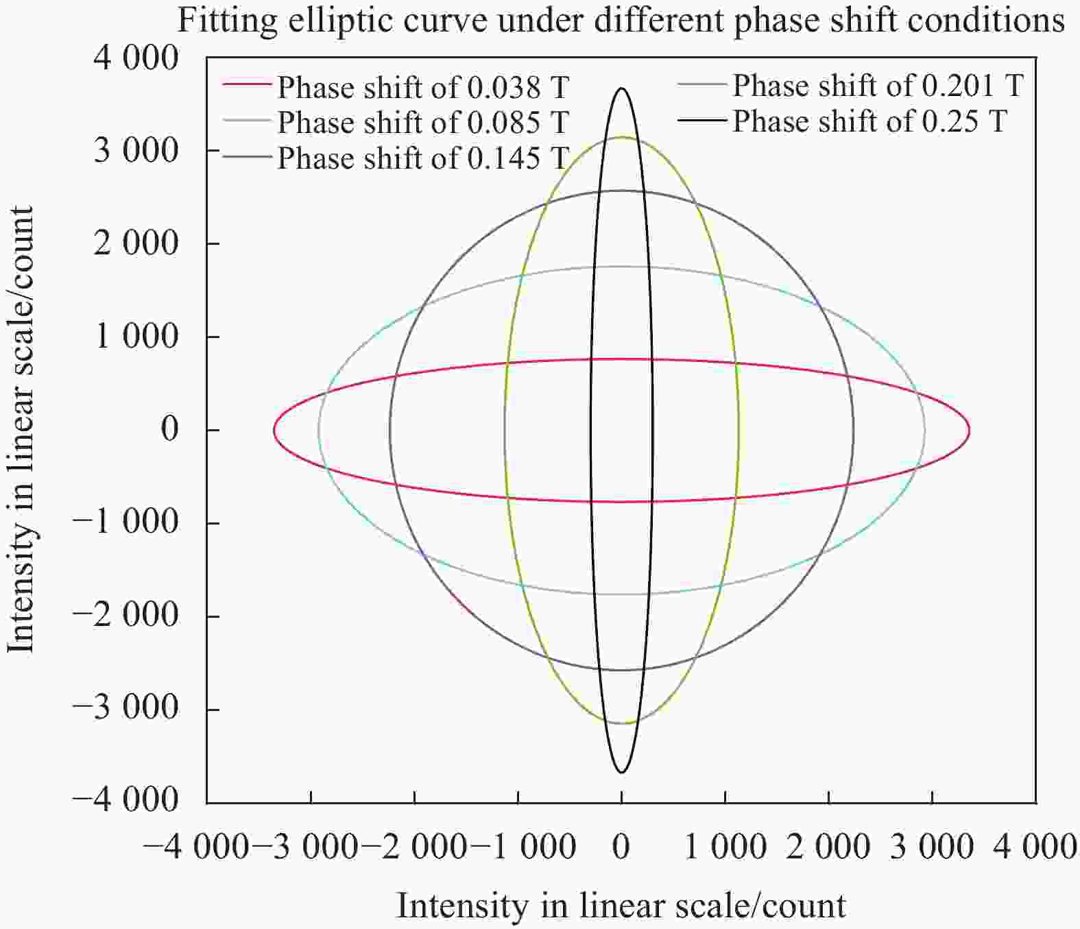
图 8 不同相移所拟合的 Lissajous 椭圆
Figure 8. Lissajous ellipse fitted by different phase shifts
-
为了验证该算法的可行性,搭建了EFPI传感器的解调实验装置,图9(a)所示为应力加载实验系统原理图。实验所采用的EFPI传感器腔长为206 μm,传感器长度为20 mm,采用Micron Optics的SI155解调仪,CML-1 H型应变力综合测试仪,BDCL-3型材料力学多功能实验台,现场装置如图9(b)所示。

图 9 (a) 应力实验系统原理图;(b) 现场装置图
Figure 9. (a) Schematic diagram of pressure experiment system; (b) Field device diagram
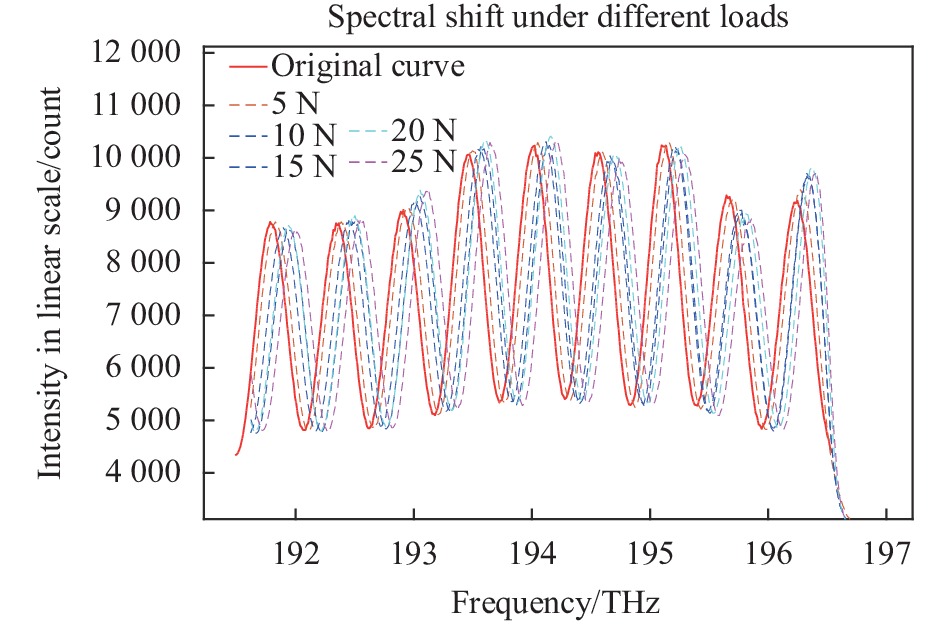
在对EFPI传感器进行横向负载实验过程中,为减小误差,均采用相移0.085 T的方式进行解调,分别施加5、10、15、20、25 N的应力所得到的光谱与原干涉谱如图10所示。

图 10 不同横向负载下EFPI输出干涉谱
Figure 10. EFPI output interference spectrum under different lateral loads
-
将实验得到的横向负载作用力下的干涉谱进行Lissajous曲线的绘制、椭圆曲线的拟合与EMD去基线处理后,解调出腔长的相关参数记录如表3所示。
表 3 不同负载条件下的腔长解调结果
Table 3. Cavity length demodulation results under different load conditions
Loads/N a/count b/count Φ/(°) d/μm $\Delta {d}_{实际}{}_{\text{actual}}$/μm $ \Delta {d}_{理论}{}_{\text{theory}} $/μm Error 0 2906.451 1118.232 42.249 206.587 5 2894.729 1128.940 42.557 207.850 1.262 1.197 5.160% 10 2880.228 1152.088 43.724 213.813 7.225 6.785 6.089% 15 2769.411 1135.451 44.023 215.995 9.408 8.934 5.041% 20 2753.020 1156.259 44.963 219.572 12.958 12.210 5.782% 25 2740.341 1164.638 45.326 223.299 16.711 15.645 6.380% 利用腔长变化量的理论计算公式进行腔长变化量的计算,可表示为:
$$ \Delta d = \varepsilon \cdot L $$ (10) 式中:L为EFPI传感器的长度,大小为20 mm;
$ \varepsilon $ 为传感器在横向负载作用力下受到的应变。取5 N力下由COMSOL仿真计算出传感器所受应变大小为5.96 e−5,由公式(10)可知,腔长变化量随负载大小成正比。由表3可知,在0~25 N范围内的横向负载作用力下,解调出的腔长平均误差为5.690%,腔长差随所施加负载增大而增大,与预期相符合。
将解调出的数据进行Lissajous图形的绘制,如图11所示,可以看出解调结果和实际相一致,解调具有良好的准确度。

图 11 不同横向负载拟合的Lissajous椭圆
Figure 11. Lissajous ellipse fitted with different transverse loads
-
依据EFPI的反射光强近似呈余弦特性,提出了一种基于标准形式椭圆参数曲线拟合的解调算法。首先通过对反射光谱进行Lissajous处理,得到的椭圆曲线为椭圆长轴与X轴呈45°的椭圆曲线,选用了速度较快的标准参数形式,在对坐标轴进行变换后,进行椭圆曲线拟合,对得到的光谱数据进行EMD分解,并在去基线之后求得光谱的极值点进而求得椭圆相关参数。利用相位处理,完成了EFPI传感器的解调,选用腔长为298 μm的EFPI传感器器,分别采用了五次相移进行解调,并用206 μm的EFPI传感器进行横向负载实验,分析了横向负载下EFPI传感器腔长的解调结果并与实际相对比,计算了两者之间的误差,验证了解调算法的精确度。但还有一些不足,比如在相移实验中,当相移超过0.3 T,解调将失去准确度,这是因为此时相移α已超过信号的周期,选取的极值点经过平移落在了下一个波峰(波谷)中。在后续的研究中,可以尝试制作更多不同腔长不同类型的EFPI传感器的进行椭圆曲线的解调,提高其精度。
Cavity length demodulation of EFPI optical fiber sensor based on Lissajous curve fitting
-
摘要: 为提高非本征光纤珐珀传感器(Extrinsic Fabry-Perot Interferometric, EFPI)腔长解调的精度,基于EFPI传感器反射光谱近似余弦函数的特性,设计了一种基于李萨如图形(Lissajous-Figure)与标准形式椭圆曲线拟合的解调方法。将两组光强信号经过坐标变换拟合为标准椭圆曲线,以减少求解参数;并通过经验模态分解对数据进行分析,去余项后将得到的极值点代入椭圆曲线求解。将离散数据点分别移动5、10、15、20、25个点测试五组不同相移对解调结果的影响并选取其中误差最小的一组对EFPI传感器进行横向负载实验,分别施加5~25 N的应力,通过拟合椭圆曲线的解调方法将计算腔长差与理论腔长差相对比。结果表明,实际腔长差随负载成正比,平均误差值为5.690%左右,可以准确获取 EFPI 的腔长。Abstract: In order to improve the accuracy of cavity length demodulation of Extrinsic Fabry-Perot Interferometric (EFPI), a demodulation method based on the approximate cosine function of the reflection spectrum was designed based on Lissajous-Figure and standard elliptic curve fitting. The two sets of light intensity signals were fitted into standard elliptic curves by coordinate transformation to reduce the required parameters; The empirical mode decomposition was used to analyze the data. The extreme point obtained after the baseline was taken into the elliptic curve to solve the problem. The discrete data points were moved by 5, 10, 15, 20 and 25 points respectively to test the influence of five groups of different phase shifts on the demodulation results, and the group with the smallest error was selected for the transverse load experiment of EFPI sensor. The stress of 5-25 N was applied respectively, the calculated cavity length difference was compared with the theoretical cavity length difference by the demodulation method of fitting elliptic curve. The results show that the actual cavity length difference is proportional to the load, the average error is about 5.690%, and the cavity length of EFPI can be obtained accurately.
-
图 4 (a) 去噪前的波峰;(b)去噪后的波峰
Figure 4. (a) Peak before denoising; (b) Peak after denoising
图 8 不同相移所拟合的 Lissajous 椭圆
Figure 8. Lissajous ellipse fitted by different phase shifts
图 9 (a) 应力实验系统原理图;(b) 现场装置图
Figure 9. (a) Schematic diagram of pressure experiment system; (b) Field device diagram
图 10 不同横向负载下EFPI输出干涉谱
Figure 10. EFPI output interference spectrum under different lateral loads
图 11 不同横向负载拟合的Lissajous椭圆
Figure 11. Lissajous ellipse fitted with different transverse loads
表 1 不同极值类型解调结果
Table 1. Demodulation results of different types of extreme values
Extreme value type a/count b/count d/μm Error Two maxima 2930.476 1752.153 309.278 3.784% Two minima 2912.415 1765.563 291.262 2.262% Maximum and minimum 2924.607 1759.400 303.951 1.993%  下载: 导出CSV
表 2 不同相移下椭圆解调结果与误差
Table 2. Elliptic demodulation results and errors under different phase shifts
Phase shift/THz a/count b/count Φ/(°) d/μm Error 0.038 3354.702 765.866 25.910 285.171 4.310% 0.085 2924.607 1759.400 61.929 303.951 1.993% 0.145 2236.514 2571.339 97.981 281.162 5.661% 0.201 1129.871 3143.681 140.429 288.461 3.208% 0.250 299.644 3669.338 170.652 285.714 4.128%
下载: 导出CSV
表 3 不同负载条件下的腔长解调结果
Table 3. Cavity length demodulation results under different load conditions
Loads/N a/count b/count Φ/(°) d/μm $\Delta {d}_{实际}{}_{\text{actual}}$ /μm$ \Delta {d}_{理论}{}_{\text{theory}} $ /μmError 0 2906.451 1118.232 42.249 206.587 5 2894.729 1128.940 42.557 207.850 1.262 1.197 5.160% 10 2880.228 1152.088 43.724 213.813 7.225 6.785 6.089% 15 2769.411 1135.451 44.023 215.995 9.408 8.934 5.041% 20 2753.020 1156.259 44.963 219.572 12.958 12.210 5.782% 25 2740.341 1164.638 45.326 223.299 16.711 15.645 6.380%
下载: 导出CSV
-
[1] 赵士元, 崔继文, 陈勐勐. 光纤形状传感技术综述[J]. 光学精密工程, 2020, 28(01): 10-29. doi: 10.3788/OPE.20202801.0010 Zhao S Y, Chui J W, Chen M M, et al. Review on optical fiber shape sensing technology [J]. Optics and Precision Engineering, 2020, 28(1): 10-29. (in Chinese) doi: 10.3788/OPE.20202801.0010 [2] 吴静红, 叶少敏, 张继清, 等. 基于光纤光栅监测技术的京雄高铁大断面隧道结构健康监测[J]. 激光与光电子学进展, 2020, 57(21): 210603. Wu J H, Ye S M, Zhang J Q, et al. Structural health monitoring of large-Section tunnel of Jing-xiong high speed railway based on fiber Bragg grating monitoring technology [J]. Laser & Optoelectronics Progress, 2020, 57(21): 210603. (in Chinese) [3] Liu F K, Cui M X, Ma J J, et al. An optical fiber taper fluorescent probe for detection of nitro-explosives based on tetraphenylethylene with aggregation-induced emission [J]. Optical Fiber Technology, 2017, 36: 98-104. doi: 10.1016/j.yofte.2017.03.004 [4] 李钧寿, 朱永, 王宁, 等. 一种提高快速光纤珐-珀非扫描式相关解调系统信号稳定性的算法[J]. 光子学报, 2015, 44(01): 91-97. Li J S, Zhu Y, Wang N, et al. An algorithm for improving the signal stability of the fast fiber optic fabry-perot nonscanning correlation demodulation system [J]. Acta Photonica Sinica, 2015, 44(1): 91-97. (in Chinese) [5] 赵文涛, 宋凝芳, 宋镜明, 等. 三波长数字相位解调法解调误差及影响因素[J]. 北京航空航天大学学报, 2017, 43(08): 1654-1661. Zhao W T, Song N F, Song J M, et al. Demodulation error and influencing factor of three-wavelength digital phasdemodulation method [J]. Journal of Beijing University of Aeronautics and Astronautics, 2017, 43(8): 1654-1661. (in Chinese) [6] Jiang X H, Tao C Y, Xiao J J, et al. Fiber-ring laser strain sensing system with two-wave mixing interferometric demodulation [J]. Acta Optica Sinica, 2021, 41(13): 1306021. (in Chinese) [7] 田培廷, 赵英亮, 王黎明, 等. 基于EFPI地声传感器的信号解调算法[J]. 光通信技术, 2020, 44(11): 20-23. Tian P T, Zhao Y L, Wang L M, et al. Signal demodulation algorithm based on EFPl geoacoustic sensor [J]. Optical Communication Technology, 2020, 44(11): 20-23. (in Chinese) [8] 何文涛, 赵光再, 宁佳晨, 等. 基于FFT和复域相关的光纤EFPI压力传感器多腔长解调方法[J]. 遥测遥控, 2019, 40(03): 17-21. He W T, Zhao G Z, Ning J C, et al. Multi-cavities demodulation algorithm of EFPl pressure based on FFT and complex domain correlation [J]. Journal of Telemetry, Tracking and Command, 2019, 40(3): 17-21. (in Chinese) [9] Jia J S, Jiang Y, Huang J B, et al. Symmetrical demodulation method for the phase recovery of extrinsic Fabry-Perot interferometric sensors [J]. Optics Express, 2020, 28(7): 9149-9157. [10] Liu Q, Jing Z G, Li A, et al. Common-path dual-wavelength quadrature phase demodulation of EFPI sensors using a broadly tunable MG-Y laser [J]. Optics Express, 2019, 27(20): 27873. doi: 10.1364/OE.27.027873 [11] 王伟, 唐瑛, 张雄星, 等. 短腔长复合式光纤法布里-珀罗压力传感器椭圆拟合腔长解调算法[J]. 光学学报, 2019, 39(6): 0606001. doi: 10.3788/AOS201939.0606001 Wang W, Tang Y, Zhang X X, et al. Elliptical-fitting cavity length demodulation algorithm for compound fiber-optic fabry-perot pressure sensor with short cavity [J]. Acta Optica Sinica, 2019, 39(6): 0606001. (in Chinese) doi: 10.3788/AOS201939.0606001 [12] 刘锋伟. 随机相移干涉测量关键技术研究[D]. 成都: 中国科学院光电技术研究所, 2017: 04-06. Liu F W. Study of key technology of random phase shifting interferometry [D]. Chengdu: Chinese Academy of Sciences, 2017: 4-6. (in Chinese) [13] 张磊磊. 基于EMD 的心电信号去噪方法研究及实现验证[D]. 重庆邮电大学, 2016 Zhang L L. ECG signal denoising method based on EMD and experimental verification[D]. Chongqing: Chongqing University of Posts and Telecommunications, 2016. (in Chinese) -

 点击查看大图

计量
- 文章访问数: 179
- HTML全文浏览量: 38
- PDF下载量: 29
- 被引次数: 0


