


 下载:
下载:


-
微波成像是一种全天时、全天候、远距离的信息获取手段,在空间监视、对地观测、安检安防等军事和民用领域有着广泛应用[1-3]。与光学成像相比,微波成像工作波长(厘米级)与光学成像(亚微米级)相差约5个数量级,受限于天线孔径尺寸,成像角分辨率远低于光学成像,极大限制了微波成像应用。自20世纪50年代以来,逐步发展了以“综合孔径”和“合成孔径”为代表的微波成像技术,提高了微波成像空间分辨率。其中,“综合孔径”采用空间占据思想,通过构建分布式天线阵列形成等效大孔径获得高的成像分辨率;而“合成孔径”采用空间遍历思想,将成像系统置于运动平台,利用平台运动形成大的虚拟合成孔径提高成像分辨率[4]。综合孔径成像需要耗费极大的空间资源,系统复杂度较高;而合成孔径成像需要平台相对目标做横向运动,适用于侧视和大斜视成像,当成像系统与目标相对静止(“凝视”)以及平台前视时,难以成像。综合来看,微波成像的一个核心问题是如何突破实际天线孔径对成像分辨率的限制,以获得高的空间分辨率。在成像系统天线孔径约束下,实现微波前视和凝视成像,成为微波成像领域的挑战性科学问题,长期以来缺乏理论支撑。由于前视和凝视成像在重点区域持续观测、无人系统目标及环境自主感知等领域具有迫切需求,突破微波前视成像瓶颈难题,发展微波成像理论受到广泛关注。
关联成像是一种基于光场高阶关联获取物体信息的主动成像技术[5]。关联成像系统采用两束具有空间关联特性的光:一束称为参考光,经自由传播后其光强空间分布被记录下来;另一束称为物臂光,经过物体后由一个没有空间分辨能力的点探测器收集(孔径内能量被透镜收集至一点,也称桶探测)。两束光通过光场强度关联处理,获得具有空间分辨能力的物体成像结果[5]。从原理上来说,关联成像是通过对照射光源的光场调制,形成具有空间涨落特性的光强分布照射物体,并与不具备空间分辨能力的单像素接收信号的强度关联重构物体图像。由于接收单元不具备分辨能力,图像重构是依靠照射光源调制获得空间分辨力,这一原理为突破天线孔径限制实现微波高分辨成像提供了重要启示:通过发射信号调制形成具有空间起伏特性的微波辐射场,通过对成像区域多次不同模式照射,采用低分辨率接收单元有望重构目标高分辨图像。
2010年以来,我国学者将光学关联成像思想引入微波成像领域,逐步发展起来一套微波关联成像理论与技术,通过实验验证了成像原理的可行性,并在应用技术研究方面取得了系列研究成果[6-15]。由于微波成像与光学成像在成像原理与实现方式上存在较大差异,微波关联成像的研究不仅拓展了经典关联成像理论,也创新发展了微波成像技术,推动了成像体制与应用的进步。文中梳理总结了微波关联成像的技术起源与发展现状,对成像原理、成像分辨率表征等基础性问题进行剖析,综述了稀疏与扩展目标、静止与运动目标以及存在各种模型失配的微波关联成像方法,阐述了随机辐射、波前调制、孔径编码等不同形态的系统体制与成像原理,比较了数字阵列、等离子体透镜、超材料等不同形式的系统实现方式,分析其中的联系与差异,厘清技术发展脉络。最后,对微波关联成像的未来发展趋势进行了总结和展望。
-
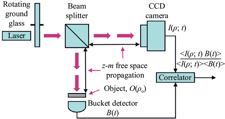
微波关联成像技术起源于光学强度关联成像。经典光学关联成像又称为鬼成像(Ghost imaging)、符合成像(Coincidence imaging)等,基于光场高阶关联来获取物体信息。最初的鬼成像实验利用了光子对的纠缠性质,后续研究发现基于纠缠光和(赝)热光均可实现关联成像[5],目前常用旋转毛玻璃、空间光调制器等器件调制相干光源,以产生具有强度涨落特性的光场,调制器件各点引入对相干光波前的随机强度或相位调制。经过分束器分成参考光和物臂光两束光路,其中,参考光被CCD记录,物臂光采用不具备空间分辨能力的桶探测器接收。根据强度涨落关联理论,将物臂光与参考光进行二阶关联实现物体图像复原,如图1所示。光学强度关联成像在提升成像抗干扰能力、提高成像分辨率等方面相比传统光学成像方法具有一定优势。
微波关联成像是通过在微波频段产生具有时变和空变特性的辐射场分布,对成像区域形成差异性照射,将目标回波信号与辐射场进行关联处理,重构目标图像。由于对目标的分辨是源于发射信号调制,打破了传统微波成像技术方位向分辨对观测视角和多普勒的依赖性,无需成像系统与目标的相对运动,有望应用于微波前视和凝视成像。相比光学关联成像,微波关联成像工作频段低、角分辨率不高,因此,更加关注成像分辨率的提升。此外,作为参考信号的微波辐射场既可以通过信号记录或测量方式得到,也可根据信号模型推演计算得出。因此,微波关联成像更易于采用计算成像方式实现,在成像处理方面可以与先进信号处理算法结合,获得成像性能提升。
-
微波关联成像借鉴光学关联成像思想,通过对发射信号调制,形成在时间和空间上具有起伏特性的随机辐射场,以模拟随机涨落特性的赝热光场分布,采用单阵元天线接收目标回波信号,将目标散射回波与随机辐射场进行关联处理,实现目标重构,成像原理如图2所示[15]。
不失一般性,考虑二维成像问题,设采用阵列方式对N个阵元发射信号幅度、频率或相位等参数进行调制,在空域合成具有强度随机涨落特性的辐射场分布,第
$n$ 个阵元发射信号记为$ {S_{{\text{T}}n}}(t) $ ,发射天线位置矢量记为${{{R}}_n}$ 。采用单阵元天线接收目标回波信号,接收信号记为$ {S_{\text{R}}}(t) $ ,接收天线位置矢量记为${{{R}}_{\boldsymbol{r}}}$ 。理想情况下,不同阵元发射信号相互正交,同一阵元发射信号在时间上不相关,即时间和空间相关函数满足[9, 16-17]:$$ R({t_1},{t_2}) = \int {{S_{{\text{T}}n}}(t - {t_1}){S_{{\text{T}}n}}(t - {t_2})} {\rm{d}}t = \delta ({t_1} - {t_2}) $$ (1) $$ R(n,m) = \int {{S_{{\text{T}}n}}(t){S_{{\text{T}}m}}(t)} {\rm{d}}t = \delta (n - m) $$ (2) 在成像区域
$ {\text{I}} $ 内,位置${{r}}$ 处的辐射信号记为${S_{\text{I}}}(t,{{r}})$ ,其中${{r}} \in {\text{I}}$ 。${S_{\text{I}}}(t,{{r}})$ 为${{N}}$ 个阵元发射信号在${{r}}$ 处的延时叠加,即:$$ {S_{\text{I}}}(t,{{r}}) = \sum\limits_{n = 1}^N {{S_{{\text{T}}n}}(t - \frac{{|{{r}} - {{{R}}_n}|}}{{c}})} $$ (3) 式中:c为光速。根据发射信号性质(1)和(2),辐射信号
${S_{\text{I}}}(t,{{r}})$ 关于时间和空间的二维相关函数为:$$ {R_{\text{I}}}(\tau ,\tau ';{{r}},{{r}}') = \int {{S_{\text{I}}}(t - \tau ,{{r}}){S_{\text{I}}}^ * (t - \tau ',{{r}}')} {\rm{d}}t \approx {{N}} \cdot \delta \left( {\tau - \tau ';{{r}} - {{r}}'} \right) $$ (4) 式中:“*”表示复信号的共轭。公式(4)表示在成像区域形成具有时间和空间独立性的辐射场分布。
目标回波信号可表示为:
$$ {S_{\text{R}}}(t) = \int_{\text{I}} {{\sigma _{{r}}}{S_{\text{I}}}\left(t - \frac{{|{{r}} - {{{R}}_r}|}}{{c}},{{r}}\right){\rm{d}}{{r}}} $$ (5) 式中:
$ {\sigma _r} $ 表示成像区域位置${{r}}$ 处的目标散射系数。将公式(5)中包含回波时延的辐射信号
$ {S_{\text{I}}} $ 记为关联成像参考信号,即:$$ S(t,{{r}}) = {S_{\text{I}}}\left(t - \frac{{|{{r}} - {{{R}}_r}|}}{{c}},{{r}}\right) $$ (6) 则目标回波信号可简化表示为:
$$ {S_{\text{R}}}(t) = \int_{\text{I}} {{\sigma _{{r}}}S(t,{{r}}){\rm{d}}{{r}}} $$ (7) 将目标回波信号与参考信号进行关联处理可得:
$$ \int {{S_{\text{R}}}(t){S^*}(t,{{r}})} {\rm{d}}t \approx {{N}} \cdot {\sigma _{{r}}} $$ (8) 因此,可以求得目标散射系数为:
$$ {\sigma _{{r}}} \approx \frac{1}{{{N}}}\int {{S_{\text{R}}}(t){S^*}(t,{{r}})} {\rm{d}}t $$ (9) 如公式(9)所示,在理想情况下,通过接收信号和参考信号之间的关联处理可以获得成像区域内任意位置处的散射信息。对于微波关联成像,由于各阵元发射信号已知,参考信号可根据发射信号以及成像几何计算得到,通过关联处理重构目标图像。与光学关联成像相比,微波关联成像可通过测量记录或计算方式获得参考信号,成像过程可通过计算方式实现。因此,微波关联成像可认为是一种计算关联成像方式。
若将时间和空间参数进行离散化表示,公式(7)也可以表示为离散形式。根据目标等效散射中心理论,光学区目标散射特性可等效为多个强散射点,将成像区域均匀划分为
${{L}}$ 个成像单元,每个单元网格中心位置矢量记为${{{r}}_l}$ ,$l = 1, \ldots ,{{L}}$ ,每个成像网格的目标等效散射系数记为${\sigma _l}$ 。将发射信号进行离散化,采样时刻记为${{t}} = {[{t_0},{t_1} \cdots {t_{{{M}} - 1}}]^{\rm T}}$ ,${{M}}$ 表示采样点数。则公式(7)可表示为矩阵形式:$$ \begin{split} &\left[ {\begin{array}{*{20}{c}} {{S_{\text{R}}}({t_0})} \\ {{S_{\text{R}}}({t_1})} \\ {...} \\ {{S_{\text{R}}}({t_{{{M}} - 1}})} \end{array}} \right] =\\ &\left[ {\begin{array}{*{20}{c}} {S({t_0},{{{r}}_1})}&{S({t_0},{{{r}}_2})}&{...}&{S({t_0},{{{r}}_{{L}}})} \\ {S({t_1},{{{r}}_1})}&{S({t_1},{{{r}}_2})}&{...}&{S({t_1},{{{r}}_{{L}}})} \\ {...}&{...}&{...}&{...} \\ {S({t_{{{M}} - 1}},{{{r}}_1})}&{S({t_{{{M}} - 1}},{{{r}}_2})}&{...}&{S({t_{{{M}} - 1}},{{{r}}_{{L}}})} \end{array}} \right] \cdot \left[ {\begin{array}{*{20}{c}} {{\sigma _1}} \\ {{\sigma _2}} \\ {...} \\ {{\sigma _{{L}}}} \end{array}} \right] \end{split}$$ (10) 若回波信号中存在测量噪声,则微波关联成像数学模型可表示为矢量形式:
$$ {{\boldsymbol{S}}_{\text{R}}} = {\boldsymbol{S}} \cdot {\boldsymbol{\sigma }} + {\boldsymbol{n}} $$ (11) 式中:
$ {{\boldsymbol{S}}_{\text{R}}} $ 表示回波信号矢量;$ {\boldsymbol{S}} $ 表示辐射场参考矩阵;$ {\boldsymbol{\sigma }} $ 表示目标散射系数矢量;$ {\boldsymbol{n}} $ 表示测量噪声矢量。回波信号矢量$ {{\boldsymbol{S}}_{\text{R}}} $ 由接收阵元采集数据得到,辐射场参考矩阵$ {\boldsymbol{S}} $ 由发射信号推演计算得出,目标散射系数矢量$ {\boldsymbol{\sigma }} $ 为待求解未知量。因此,微波关联成像可以建模为一个线性模型,成像重构可以视为线性逆问题的求解。根据辐射场参考矩阵
$ {{{\boldsymbol{S}}}} $ 以及目标散射系数矢量${{{\boldsymbol{\sigma}} }}$ 的性质,可以采用多种求解方法获得目标散射系数矢量${{{\boldsymbol{\sigma}}}}$ 的估计,从而重构目标图像。成像数学模型(11)通常也称为微波关联成像方程。 -
根据微波成像理论,传统微波成像的距离和方位向空间分辨率分别由发射信号带宽和天线有效孔径决定,即
$$ \left\{ \begin{gathered} {\rho _r} = \frac{{c}}{{2B}} \hfill \\ {\rho _\varphi } = \frac{\lambda }{D} \cdot R \hfill \\ \end{gathered} \right. $$ (12) 式中:B为发射信号带宽;
$ c $ 为光速;$ \lambda $ 为发射信号波长;D为成像的有效天线孔径;R为成像距离。当发射信号波长确定时,方位向分辨率取决于天线孔径尺寸。由于微波关联成像原理与传统微波成像技术有较大不同,成像分辨率与辐射场参考矩阵
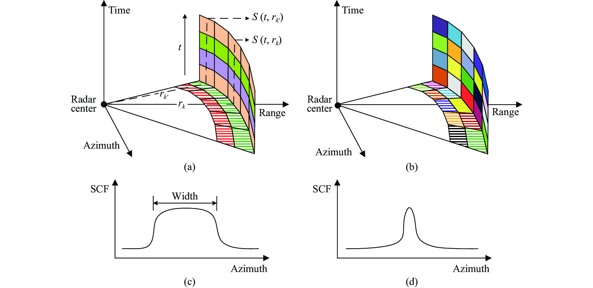
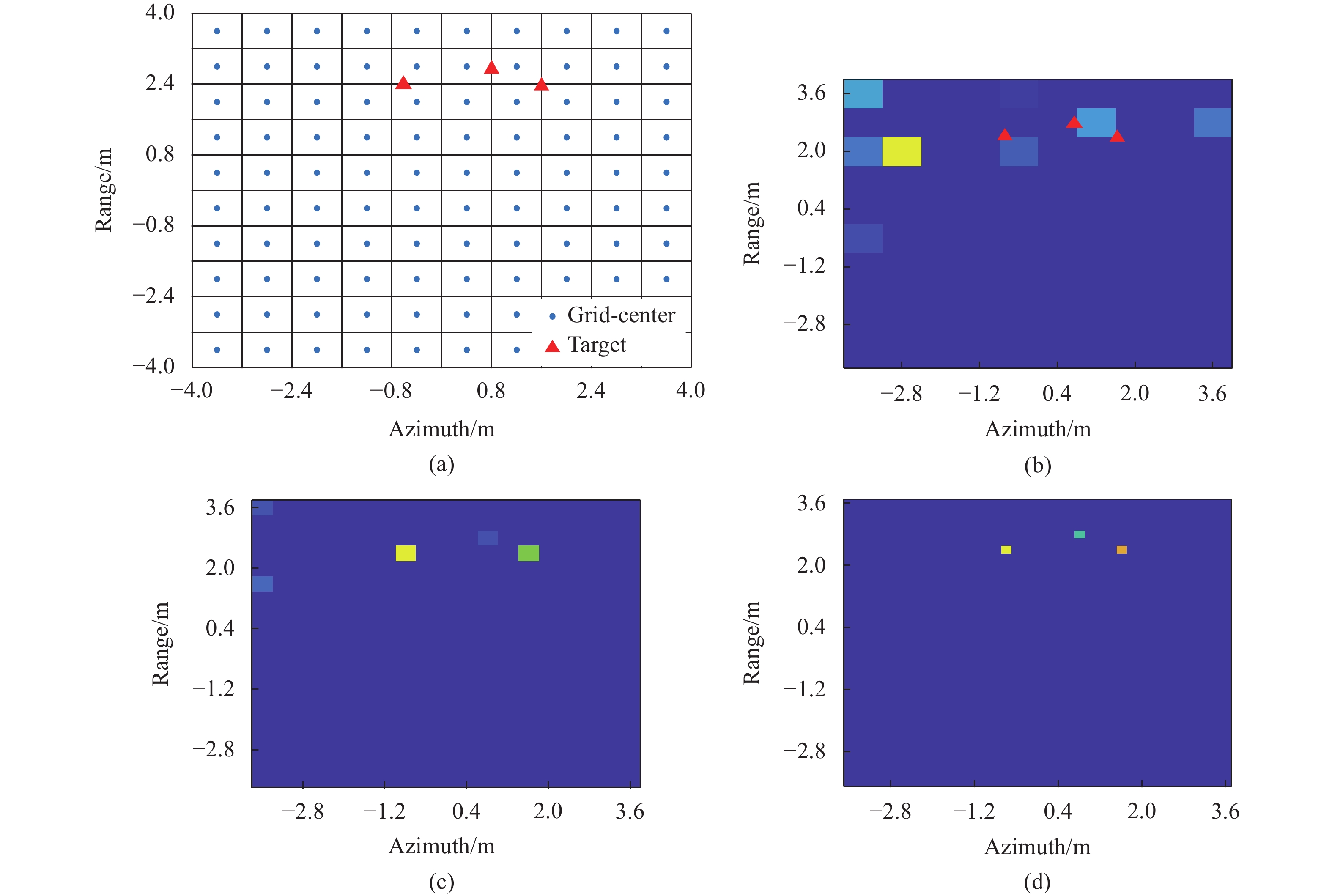
$ {\boldsymbol{S}} $ 、目标散射系数分布$ {\boldsymbol{\sigma }} $ 以及求解方法等都存在联系。因此,难以给出解析的分辨率表达式,不过,通过对各种影响因素的分析,可以给出理论估计值。微波关联成像分辨率表征示意图如图3所示。其中,传统成像技术在空域发射相干信号,不同方位向信号具有较强相关性,而关联成像在空域发射时间和空间不相关的辐射信号,不同方位向信号相关性较弱。为了对成像分辨率进行定量分析,定义方位向两个相邻位置
$ {{{r}}_k} $ 和$ {{{r}}_{k'}} $ 的空间相关函数为[15]:
图 3 微波关联成像分辨率表征[15]。(a) 传统成像相干发射情形;(b) 关联成像非相干发射情形;(c) 传统成像空间相关函数;(d) 关联成像空间相关函数
Figure 3. Resolution analysis of microwave coincidence imaging[15]. (a) Coherent transmissions of conventional imaging; (b) Incoherent transmissions of coincidence imaging; (c) Spatial correlation function of conventional imaging; (d) Spatial correlation function of coincidence imaging
$$ \chi \left( {{{{r}}_k},{{{r}}_{k'}}} \right) = \frac{{\left| {\left\langle {S\left( {t,{{{r}}_k}} \right),S\left( {t,{{{r}}_{k'}}} \right)} \right\rangle } \right|}}{{\left\| {S\left( {t,{{{r}}_k}} \right)} \right\|\left\| {S\left( {t,{{{r}}_{k'}}} \right)} \right\|}} $$ (13) 式中:
$\left\langle {S\left( {t,{{{r}}_k}} \right),S\left( {t,{{{r}}_{k'}}} \right)} \right\rangle$ 表示关于时间$ t $ 的集合平均;$ \left\| \cdot \right\| $ 表示矩阵范数。空间相关函数给出了辐射场参考信号
$S(t,{{r}})$ 时间和空间相关性的度量,与成像分辨率存在紧密联系。当两个相邻位置的参考信号$ S\left( {t,{{{r}}_k}} \right) $ 和$ S\left( {t,{{{r}}_{k'}}} \right) $ 完全相关时,空间相关函数$ \chi \left( {{{{r}}_k},{{{r}}_{k'}}} \right) $ 取最大值,当二者完全不相关时,空间相关函数$ \chi \left( {{{{r}}_k},{{{r}}_{k'}}} \right) = 0 $ 。在理想情况下,当辐射场完全随机起伏时,空间相关函数为冲激函数$ \chi \left( {{{{r}}_k},{{{r}}_{k'}}} \right) = \delta \left( {{{{r}}_k} - {{{r}}_{k'}}} \right) $ 。通常,辐射场空间相关函数随方位向距离$ d = \left\| {{{{r}}_k} - {{{r}}_{k'}}} \right\| $ 增大而减小,其主瓣宽度与关联成像空间分辨率有关。为了描述关联成像空间分辨率,辐射场空间相关函数的主瓣宽度可由门限
${\chi _{{\rm{th}}}}$ 确定。若$\chi \left( {{{{r}}_k},{{{r}}_{k'}}} \right) > {\chi _{{\rm{th}}}}$ ,则两个相邻散射点信号具有较强相关性,不能分辨。临界分辨率可表示为:$$ {\rho _\varphi } = \left\| {{{{r}}_k} - {{{r}}_{k'}}} \right\| , {\text{s}}{\text{.t}}{\text{. }}\chi \left( {{{{r}}_k},{{{r}}_{k'}}} \right) = {\chi _{{\rm{th}}}} $$ (14) 其中,成像固有分辨能力由发射信号形成的辐射场空间相关函数决定,而分辨率门限
${\chi _{{\rm{th}}}}$ 与目标散射系数分布以及成像方法有关。不同发射波形对辐射场起伏程度以及空间相关函数的影响不同。图4(a)~(f)给出了随机调频、随机调幅和随机调相三种典型波形形成的辐射场及空间相关函数图。其中,发射阵列为均匀线阵,阵元个数为10,阵元间距为0.5 m,发射信号中心频率为9.5 GHz,带宽为500 MHz,辐射场平面与发射阵列距离为1 km。从图中可以看出,随机调频和随机调幅波形形成的辐射场比随机调相波形具有更强的起伏特性,空间相关函数主瓣较窄,其成像分辨率较高。

图 4 不同发射波形的空间相关函数[9]。(a)~(b) 随机调频波形辐射场和空间相关函数;(c)~(d) 随机调幅波形辐射场和空间相关函数;(e)~(f) 随机调相波形辐射场和空间相关函数
Figure 4. Spatial correlation functions of transmitted waveforms[9]. (a)-(b) Radiation field and spatial correlation function of random frequency modulation waveform; (c)-(d) Radiation field and spatial correlation function of random amplitude modulation waveform; (e)-(f) Radiation field and spatial correlation function of random phase modulation waveform

除了采用空间相关函数表征微波关联成像的固有名义分辨率,还可以采用统计分辨力[17]、平均模糊函数[18]等定义微波关联成像分辨能力。基于目标位置估计,子空间投影分辨率表征方法[19]给出了成像分辨率的一般性表述,并对成像分辨率的各种影响因素进行分析。根据线性方程组求解理论,从对公式(11)表示的微波关联成像数学模型求解的角度出发,有效秩理论可以在一定程度上反映求解的性能及成像重构的超分辨性能。
-
理论研究表明,采用二阶关联处理比一阶关联处理成像分辨率提高约55%[19]。为了进一步提高微波关联成像分辨率,基于公式(11)的成像模型,已提出多种成像方法,通过减小成像单元尺寸,细分目标散射分布,获得超分辨性能。然而,当成像单元尺寸减小时,相邻网格辐射场之间的差异性减弱,相关性增大,矩阵方程趋于病态,将求解稳定性变差。辐射场参考矩阵的有效秩可反映辐射场的相关特性[17],定量表征信号参数、成像单元尺寸以及目标复杂度等对成像重构的影响及限制性要求。
图5给出了辐射场参考矩阵有效秩随成像单元尺寸变化的关系曲线。成像区域划分为
$ 30 \times 30 $ 个成像单元,成像单元尺寸$0.2\;{\text{m}} \leqslant \Delta \leqslant 2\;{\text{m}}$ 。增大成像单元尺寸,相邻单元辐射场信号差异性提高,辐射场参考矩阵有效秩增大,当有效秩与成像单元个数相近时,辐射场参考矩阵为满秩,此时独立方程个数等于目标散射系数参数个数,目标图像可通过矩阵求逆稳健重构,此时成像分辨率由成像单元尺寸确定。理论上,提高工作频率、增大天线孔径、增大发射信号带宽,均可提高辐射场的空间差异性,增大辐射场参考矩阵有效秩,从而获得更高成像分辨率。 -
微波关联成像数学模型表明,成像重构是一个由矩阵方程描述的线性逆问题求解过程。由于实际的成像系统难以产生具有完全不相干特性的辐射场,而观测向量维度M通常小于成像单元个数L,因此,微波关联成像模型通常是一个病态的逆问题[20]。在不存在模型误差的理想情况下,理论上可以采用相关法、最小二乘法、正则化方法和压缩感知等基本成像方法重构目标图像。在实际情况下,当存在系统误差、信号误差、成像单元网格失配、目标运动失配等模型失配误差时,需要克服失配影响,存在各种模型失配情况下的稳健重构方法是微波关联成像算法研究的一个重点。
-
根据关联成像思想,目标散射系数矢量可以通过关联处理得到,即
$$ \hat{{\boldsymbol\sigma} }={{\boldsymbol{S}}}^{{\rm{H}}}\cdot{{\boldsymbol{S}}}_{\text{R}} $$ (15) 式中:
${\rm{H}}$ 表示矩阵的共轭转置。公式(15)所示的相关法直接将接收信号与辐射场参考矩阵进行相关,属于一阶关联处理,与传统微波成像中的匹配滤波处理一致。相关法可以避免由成像方程的病态所导致的求解不稳定现象,理论上成像结果无法获得超分辨效果。当存在测量噪声时,${{\boldsymbol{S}}}^{{\rm{H}}}\cdot{{\boldsymbol{S}}}_{\text{R}}\approx {{\boldsymbol{S}}}^{{\rm{H}}}\cdot\left({{\boldsymbol{S}}}_{\text{R}}+{\boldsymbol{n}}\right)$ ,由于测量噪声通常与辐射场不相关,所以相关法的优势是对测量噪声的容忍能力较强,成像结果较稳健。 -
最小二乘估计将成像模型转化为一个最小二乘问题进行求解,即:
$$ \hat{{{\boldsymbol\sigma}} }=\arg\underset{{{\boldsymbol\sigma}} }{\min}{\Vert {{{\boldsymbol S}}}_{\text{R}}-{{\boldsymbol S}}\cdot{{\boldsymbol\sigma}} \Vert }_{2}^{2} $$ (16) 最小二乘法得到的目标散射系数估计量可表示为[21]:
$$ \hat{{{\boldsymbol\sigma}} }={{{\boldsymbol S}}}^{\dagger}\cdot{{{\boldsymbol S}}}_{\text{R}} $$ (17) 式中:
${{{\boldsymbol S}}^\dagger } = {\left( {{{{\boldsymbol S}}^{\rm{H}}}{{\boldsymbol S}}} \right)^{ - 1}}{{{\boldsymbol S}}^{\rm{H}}}$ 是${{\boldsymbol S}}$ 的伪逆[22]。最小二乘法可以提高目标的成像分辨率,但对模型误差较敏感。此外,最小二乘法的性能也受到辐射场特性的约束。对于线性模型(16),在高斯噪声情况下,最小二乘估计(17)为最佳估计。最小二乘法具有一定的抗噪能力,但是要利用公式(17)对方程求解的一个必要条件是矩阵
${{\boldsymbol{S}}^{\rm{H}}}{\boldsymbol{S}}$ 可逆,当辐射场参考矩阵${\boldsymbol{S}}$ 不是满秩、条件数(Condition number)较大时,成像效果不理想。辐射场参考矩阵${\boldsymbol{S}} $ 的条件数$ {N_{{\text{cond}}}} $ 定义为[23]:$$ {N}_{\text{cond}}=\Vert {{\boldsymbol S}}\Vert \cdot\Vert {{{\boldsymbol S}}}^{-1}\Vert =\frac{{\xi }_{\mathrm{max}}}{{\xi }_{\mathrm{min}}} $$ (18) 式中:
$ {\xi _{\max }} $ 和$ {\xi _{\min }} $ 分别表示${{\boldsymbol S}}$ 的最大和最小奇异值。辐射场参考矩阵
${{\boldsymbol S}}$ 的条件数取决于辐射场的非相干特性,条件数越大,非相干性越弱。空间上距离越靠近的两个位置,辐射场的相关性越强,因此当成像单元划分越细时,对应的矩阵条件数越大,导致最小二乘算法求解不稳定。条件数大的参考矩阵对应的成像方程大多属于病态方程,此时测量数据的微小扰动都可能引起求解结果产生较大误差。而条件数接近1时矩阵是良态的,此时方程求解误差对模型扰动敏感性较弱。因此,最小二乘法适用于辐射场参考矩阵${\boldsymbol{S}}$ 非相干特性较好的情况,而相关法则是对最小二乘方法中的不稳定部分作了近似处理,使求解更加稳定[24]。 -
在实际成像处理中,辐射场参考矩阵
${{\boldsymbol S}}$ 通常不是满秩的,最小二乘法的求解效果不理想,主要原因是矩阵${{{\boldsymbol S}}^{\rm{H}}}{{\boldsymbol S}}$ 求逆不稳定。作为对最小二乘法代价函数${\Vert {{{\boldsymbol S}}}_{\text{R}}-{{\boldsymbol S}}\cdot{{\boldsymbol\sigma}} \Vert }_{2}^{2}$ 的改进,Tikhonov正则化方法修正了代价函数,$$ J({{\boldsymbol\sigma}} )=\mathrm{arg}\;\underset{{{\boldsymbol\sigma}} }{\mathrm{min}}\left({\Vert {{{\boldsymbol S}}}_{\text{R}}-{{\boldsymbol S}}\cdot{{\boldsymbol\sigma}} \Vert }_{2}^{2}+\eta {\Vert {{\boldsymbol\sigma}} \Vert }_{2}^{2}\right) $$ (19) 式中:
$ \eta $ 称为正则化参数,求解方法称为Tikhonov正则化法[25-26]。其解可表示为:$$ {\hat{\boldsymbol \sigma }} = {\left( {{{{\boldsymbol S}}^{\rm{H}}}{{\boldsymbol S}} + \eta {{I}}} \right)^{ - 1}}{{{\boldsymbol S}}^{\rm{H}}}{{\boldsymbol S}_{\text{R}}} $$ (20) Tikhonov正则化方法的本质是通过对秩亏矩阵
${{{\boldsymbol S}}^{\rm{H}}}{{\boldsymbol S}}$ 每一个对角元素加一个微小的扰动参数$ \eta $ ,使得对接近奇异的协方差矩阵${{{\boldsymbol S}}^{\rm{H}}}{{\boldsymbol S}}$ 求逆变成非奇异矩阵${{{\boldsymbol S}}^{\rm{H}}}{{\boldsymbol S}} + \eta {{I}}$ 的求逆,从而提高求解的稳定性。 -
电磁散射理论表明,目标在高频区的后向散射特性可由散射中心模型描述[27],目标的散射特性可以近似为某些局部位置的散射中心响应的合成,这些局部性的散射源称为目标等效散射中心。目标等效散射中心通常具有稀疏分布特性,利用目标散射的稀疏性可以提高成像质量。在数学上,微波关联成像模型与压缩感知模型具有相似性,因此,采用压缩感知方法实现目标图像重构也是关联成像处理的一个途径。这类算法利用目标散射中心分布的稀疏先验,在测量数据有限的情况下,准确求解出
${{\boldsymbol\sigma }}$ ,此外还可以克服相关法宽主瓣和高旁瓣问题,抑制虚假散射点,提高成像质量。根据压缩感知理论,若$ {\boldsymbol{\sigma }} $ 稀疏,以下优化问题能准确求解[28]:$$ \hat{{{\boldsymbol\sigma}} }=\mathrm{arg}\;\underset{{{\boldsymbol\sigma}} }{\mathrm{min}}\left\{{\Vert {{{\boldsymbol S}}}_{\text{R}}-{{\boldsymbol S}}\cdot{{\boldsymbol\sigma}} \Vert }_{2}^{2}+\eta {\Vert {{\boldsymbol\sigma}} \Vert }_{0}\right\} $$ (21) 然而,上述
$ {\ell _0} $ 范数求解是一个NP难问题[29]。通过近似处理能够求解该问题,最常用的方法是用$ {\ell _1} $ 范数代替$ {\ell _0} $ 范数[28, 30]:$$ \hat{{{\boldsymbol\sigma}} }=\mathrm{arg}\;\underset{{{\boldsymbol\sigma}} }{\mathrm{min}}\left\{{\Vert {{{\boldsymbol S}}}_{\text{R}}-{{\boldsymbol S}}\cdot{{\boldsymbol\sigma}} \Vert }_{2}^{2}+\eta {\Vert {{\boldsymbol\sigma}} \Vert }_{1}\right\} $$ (22) 公式(22)是一个凸优化问题[31],其思想是在满足成像方程约束的前提下,求得目标稀疏解。当存在测量噪声时,问题转化为成像误差在一定范围内,使目标最稀疏。压缩感知重构方法通常具有较高的计算复杂度。
当存在测量噪声时,采用贝叶斯方法通常能够降低噪声影响,在逆问题求解时以概率形式考虑因测量噪声带来的不确定性和误差,利用先验信息和测量数据获得对未知参数的估计。贝叶斯方法与稀疏表示理论结合而发展的稀疏贝叶斯方法能够充分利用测量数据的先验信息,在目标散射系数服从某一稀疏先验分布
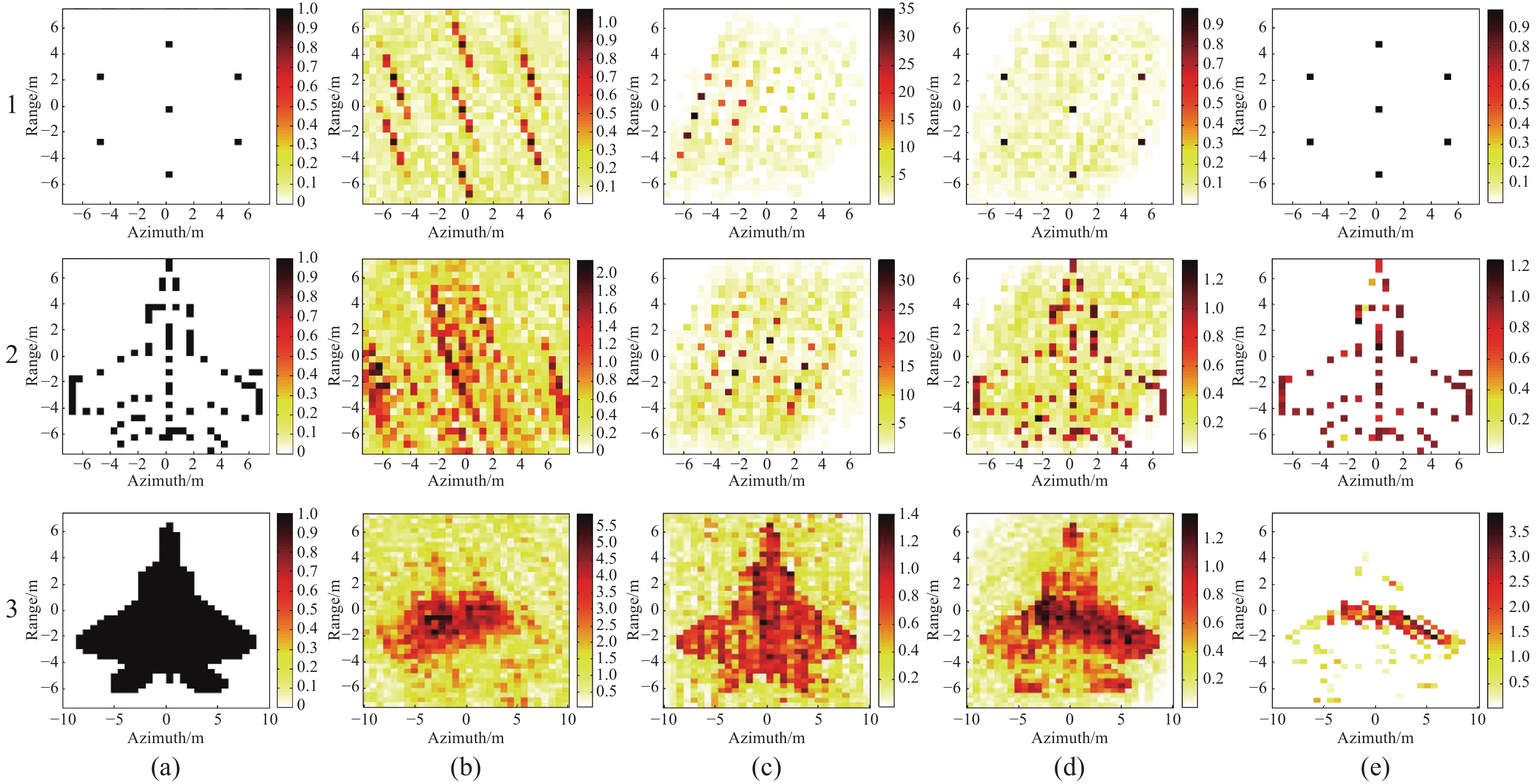
$p\left( {\boldsymbol{\sigma }} \right)$ 时,根据贝叶斯原理得出散射系数的后验概率估计。稀疏贝叶斯重构方法的目标函数可以表示为:$$ \hat{{{\boldsymbol\sigma}} }=\mathrm{arg}\;\underset{{{\boldsymbol\sigma}} }{\mathrm{max}}\;\mathrm{log}\left(p\left({{{\boldsymbol S}}}_{\text{R}}|{{\boldsymbol\sigma}} \right)\cdot p\left({{\boldsymbol\sigma}} \right)\right) $$ (23) 微波关联成像中常用的压缩感知求解方法主要有正交匹配追踪(Orthogonal matching pursuit, OMP)算法[32]、基追踪(Basis persuit, BP)算法[31]、稀疏贝叶斯学习(Sparse Bayesian learning, SBL)算法[33]等。图6给出了三种不同目标复杂度情况下,相关法、最小二乘法、Tikhonov正则化方法和SBL成像结果。其中,相关法和最小二乘法的成像质量较差,Tikhonov正则化法对矩阵求逆过程做了改进,成像质量有所提高。当目标稀疏度较高时,SBL法的成像结果较好,但不适用于复杂扩展目标成像。

图 6 各种微波关联成像算法结果对比。(a) 目标场景;(b) 相关法;(c) 最小二乘法;(d) Tikhonov正则化方法;(e) SBL
Figure 6. Comparison of various algorithms of microwave coincidence imaging. (a) Target scene; (b) Correlation; (c) Least square; (d) Tikhonov regularization; (e) SBL
-
第3.1节中所述基本成像算法只考虑了测量噪声影响,适用于关联成像模型准确情况下的目标重构。在实际中,系统误差、目标运动等会造成成像模型误差,模型失配对成像重构的准确性和成像质量有较大影响,是关联成像处理中的一个重要问题。
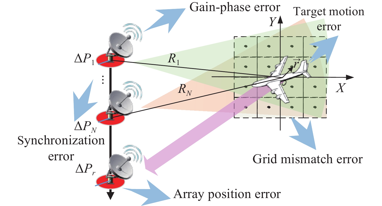
从微波关联成像处理过程可知,在关联处理前需要首先获取辐射场参考矩阵,这就需要成像模型各参数精确已知。但在实际成像过程中,普遍存在各种模型误差,如阵元间时间同步误差[34-35]、阵元位置误差[36-37]、信号幅相误差[38-42]、目标散射中心网格失配误差[43-44]和目标运动引起的失配误差[18]等,如图7所示。相比于加性噪声,模型误差引起的辐射场参考矩阵误差是一类乘性误差,建模更加复杂,对成像质量的影响也更大。
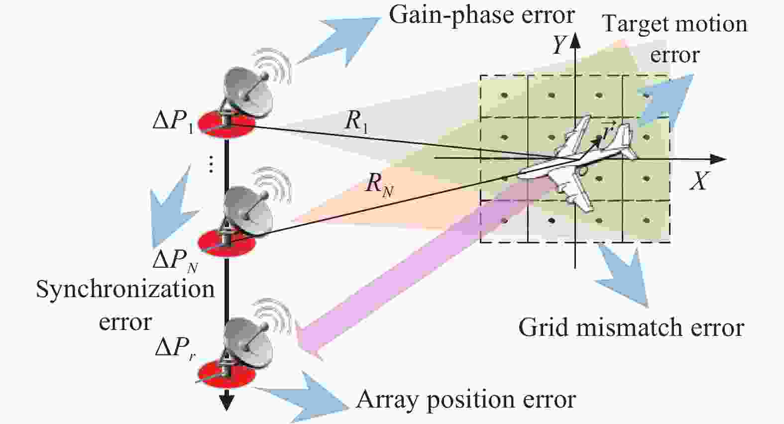
图 7 微波关联成像中各种模型失配误差示意图
Figure 7. The model error in microwave coincidence imaging
(1)针对阵元间时间同步误差,通过分析随机辐射场参考信号和回波之间的时间同步误差对微波关联成像质量的影响,基于随机辐射场短时积累的微波关联成像方法采用“脉内积累、关联处理”方式降低了时间同步误差带来的不利影响,提高了成像质量[34]。基于分时累积的图像重构方法则通过一定时间的辐射场空间差异性积累,降低了对时间同步精度的要求[35]。
(2)针对阵元位置误差,通过建立存在阵元位置误差的微波关联成像模型,推导存在阵元位置误差的散射系数估计下界CRLB,同时结合参数估计和辅助物校正、自校正等方法,在稀疏重构框架下的辅助目标校正法、迭代补偿以及等效补偿等方法能够较好地解决阵元位置误差带来的影响[16, 36-37]。
(3)针对信号幅相误差,基于凸优化理论和相位恢复算法,基于压缩感知的阵列幅相误差估计方法可对信号幅度误差和相位误差进行估计和校正[38]。基于辅助阵元的微波关联成像幅相误差校正方法,能够分别估计幅度和相位误差并进行补偿,从而获得准确的辐射场参考矩阵[42]。
(4)针对目标散射中心网格失配误差,已提出多种成像方法。在关联成像处理时,通常将成像平面划分为若干个成像单元,并假设目标散射中心位于成像单元网格中心处,但实际目标散射中心不可避免与划分的虚拟网格中心存在偏差[43-44],从而形成成像模型误差。针对网格失配问题,相关法与参数化方法联合重构能够降低模型失配误差的敏感性[9, 44]。从贪婪迭代求解和贝叶斯统计优化思路出发,基于迭代
$ {\ell _0} $ 范数的最小二乘成像算法和基于迭代最大后验的稀疏自适应校正反演方法能够对网格失配误差进行有效估计和校正[8]。前者是采用多分辨率策略更新辐射场矩阵,达到搜索校正网格失配误差的效果,后者是通过赋予散射系数和网格失配误差先验分布,从最大后验概率出发同时估计散射系数和失配误差。基于结构特征的稀疏总体最小二乘方法能够对网格失配进行校正,并利用FOCUSS方法对目标进行重构[45]。此外,不同于固定网格成像方法,多重网格划分成像方法[46-47]和动态网格划分成像方法[48-49]按照一定策略使网格迭代更新进化,从而能够使网格更好地聚集在散射点附近,有效减小网格失配误差并提高成像效率。基于瀑布型多重网格的处理方法首先对成像方程进行预处理,将原问题分解到多级疏密程度不同的网格空间,然后依次进行求解,以此来解决大场景下成像方程规模大的问题[46]。基于目标分布的非均匀网格处理方法对成像区域进行非均匀网格划分从而利用较少的网格实现对大成像场景的成像[47]。定向网格分裂成像方法将参考矩阵关于网格坐标的一阶导数加入成像模型中,并根据一阶导数确定新网格的位置,从而使网格位置更加靠近目标散射点,减小成像网格失配误差[48]。迭代重加权动态网格成像方法能够在迭代中不断细化网格,并将散射系数值作为权重值作用到网格上,从而能够剔除冗余网格,使网格聚集于目标散射点附近,在减小网格失配误差的同时提高成像效率[49],如图8所示。

(5)针对目标运动引起的失配误差,中国科学技术大学[8, 45, 50]和国防科技大学[9, 18]开展了相关算法研究。处理思路包括两种:一是基于高精度运动补偿的运动目标关联成像,通过对目标运动参数进行高精度估计,更新辐射场参考矩阵,实现运动目标重构;二是基于多维联合重构的运动目标关联成像,建立包含目标运动参数和目标散射系数的关联成像方程,通过迭代求解,对目标运动参数和目标散射系数进行联合估计。基于更新过完备字典的方法和基于速度估计的自适应稀疏反演方法能够较好地对运动目标进行成像[8];基于速度预估计的运动目标成像方法先采用相关法估计目标运动速度,然后对辐射场矩阵进行运动速度补偿[50];此外,基于参数化字典学习的自适应稀疏反演算法把对目标运动速度和目标位置的求解问题转换为连续参数估计问题,对经典SBL算法进行修改,引入运动目标速度的估计,迭代得到目标图像和运动速度[50-52]。对于静止平台,通过对目标运动状态分析获取目标速度和加速度信息,然后选择合适的观测矩阵进行成像[45];对于运动平台,关联成像体制下的目标角度获取和跟踪算法能够以先跟踪后成像的方式对动目标进行成像[18]。
-
随着微波关联成像技术研究的深入,对成像原理的认识与理解也在逐步深化,呈现出随机辐射、波前调制、孔径编码等多种理解,发展出不同形态的系统体制,形成了数字阵列、等离子体透镜、超材料等多种形式系统实现方式。此节重点阐述典型的微波关联成像系统体制及代表性系统实现方式,并介绍相关实验进展。
-
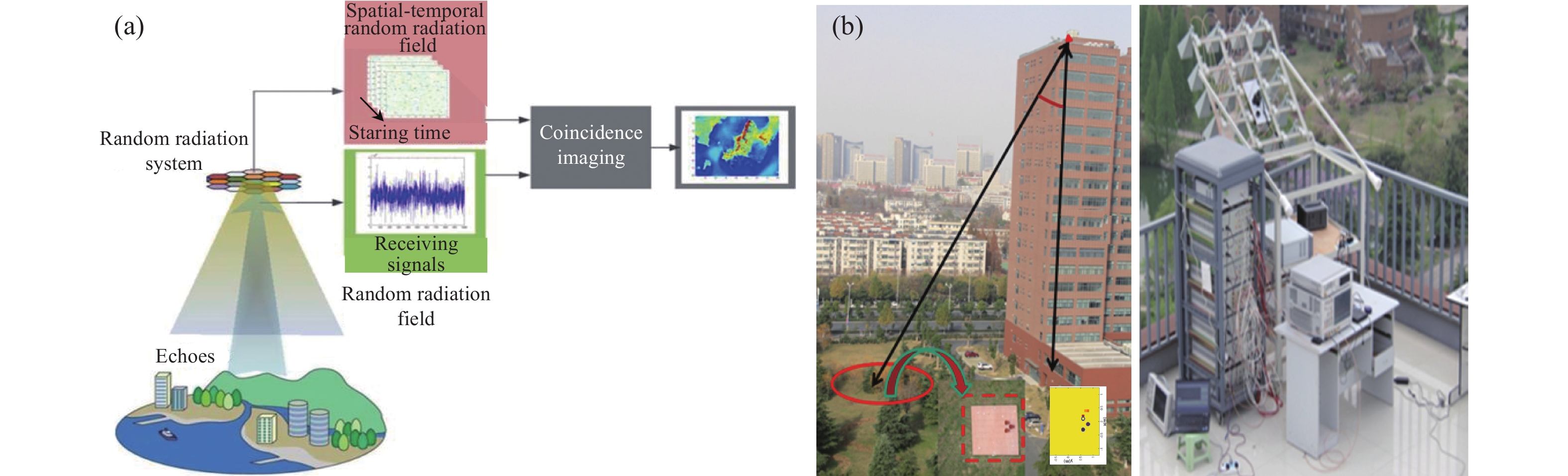
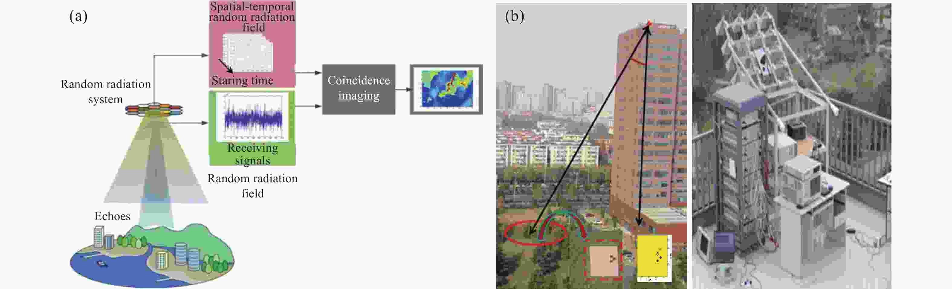
2010年,中国科学技术大学联合中国科学院上海光学精密机械研究所将光学强度关联成像思想引入微波成像,提出微波凝视关联成像概念[6-7]。基于时、空两维随机辐射场,建立了微波“随机辐射,关联成像”理论框架,从电磁场理论出发剖析微波关联成像技术的原理,揭示随机辐射场的一般统计表征规律,在微波凝视关联成像超分辨机理、随机辐射场的形成原理、随机辐射源优化设计及关联重构方法等方面开展了研究[8, 35, 45-47, 50, 53]。2013年,研制成功微波凝视关联成像原理验证实验装置,完成了楼顶平台对点目标微波凝视关联成像实验,成像距离100 m、成像分辨率超阵列实孔径10倍,初步验证了微波凝视关联成像理论的可行性,如图9所示。
中国电子科技集团公司第五十一研究所[12]、西安电子科技大学[13]、西安交通大学[14]、上海交通大学[54]、中国科学院光电研究院[55]等单位也相继开展了微波关联成像理论与技术研究。2014年,中国电子科技集团公司第五十一研究所采用单频点连续波随机移相体制,在室内静态成像实验中获得了超阵列实孔径4.5倍的成像结果。2015年,开展了单频多点接收的微波关联成像试验,实现了室外150 m距离平行腔体目标的成像。西安电子科技大学[10-11, 38]采用相控阵随机移相方式产生二维随机辐射场,对辐射源天线阵列构型和发射信号形式进行相关研究,提出了基于多阵元稀疏排布阵列构型的关联成像方法,实现稀疏目标的关联成像,通过数值仿真和微波暗室实验,获得了超阵列实孔径3倍的成像结果。
-
2012以来,国防科技大学对微波关联成像理论与应用技术开展持续研究。围绕微波前视、凝视成像瓶颈难题,从电磁波信息调制与反演角度出发,提出了微波波前调制成像理论,在微波前视成像原理、目标重构方法、成像系统研制与成像实验等方面取得系统性理论与技术成果[9, 18, 56-63],研制了国内首套微波波前调制前视成像系统[15]。

图 10 微波波前调制成像原理
Figure 10. Principle of microwave wavefront modulation imaging
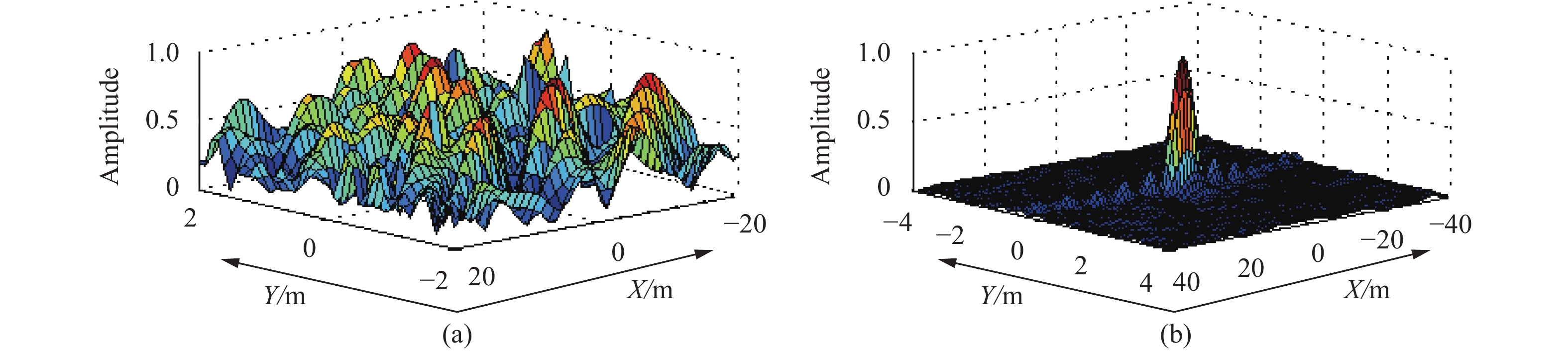
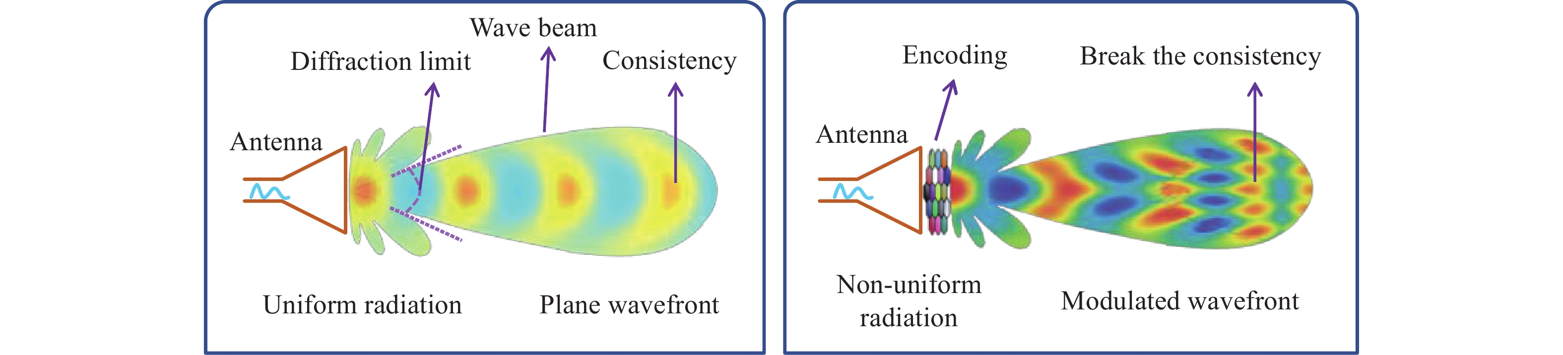
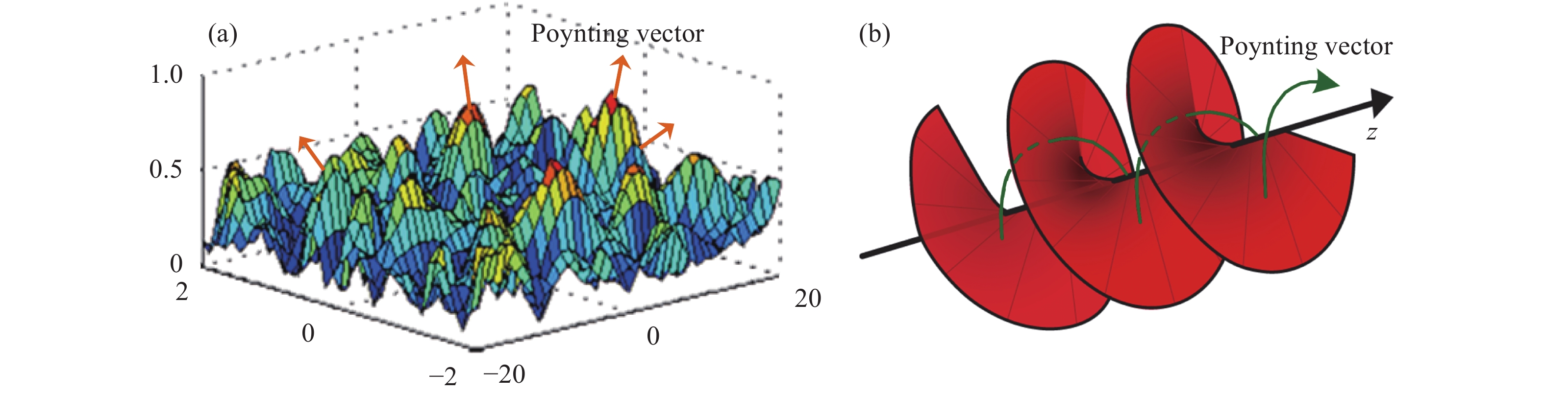
波前是电磁波传播过程中等相位面组成的曲面,不同的波前形式蕴含了不同的信息。2014年,国防科技大学提出微波波前调制概念,根据信息获取的实际需求设计复杂多变的波前。进一步,通过对电磁波波前的调控,形成具有不同波前形式的辐射模式,打破照射波束内电磁辐射信息的“同一性”,使得电磁波在不同位置处形成差异性的电磁激励,波束内目标被差异性的电磁激励所标度,通过对目标散射重构实现高分辨成像,如图10所示。根据电磁波波前调制形式的不同,研究了随机波前和涡旋波前两种典型波前调制形式,如图11所示。其中,随机波前具有最大的空间差异性,理论上信息承载能力最强,分辨能力最高[9, 18, 60-61];涡旋波前随空间方位角线性变化,呈现出周期性的相位梯度规律,便于信息处理[62-63]。分别对两种波前的产生、发射、接收及成像处理方法进行了系统研究,形成了一套微波波前调制成像理论。
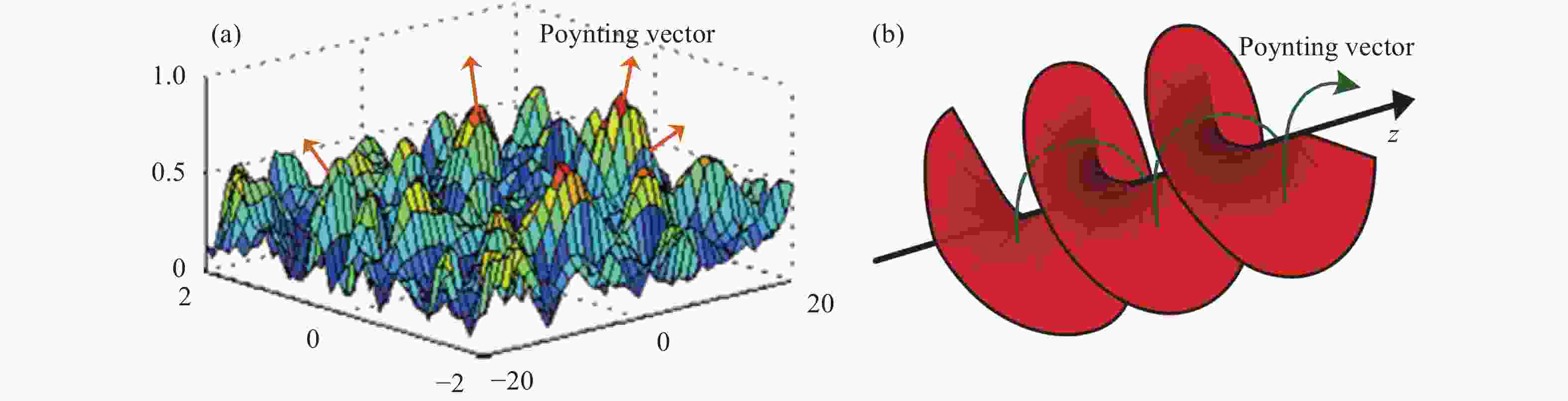
图 11 典型波前调制形式。(a) 随机波前;(b) 涡旋波前
Figure 11. Typical wavefront modulation forms. (a) Random wavefront; (b) Vortex wavefront
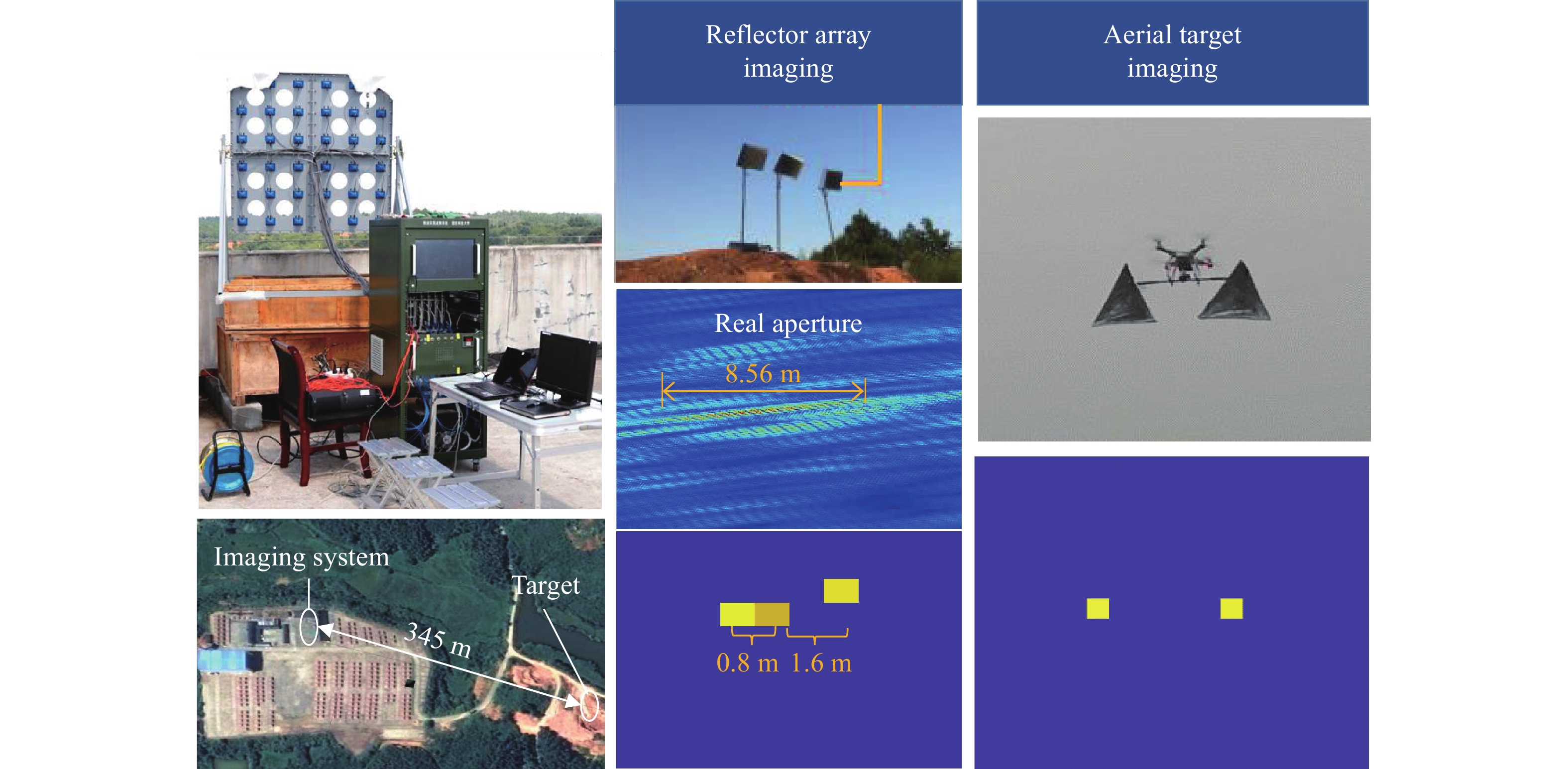
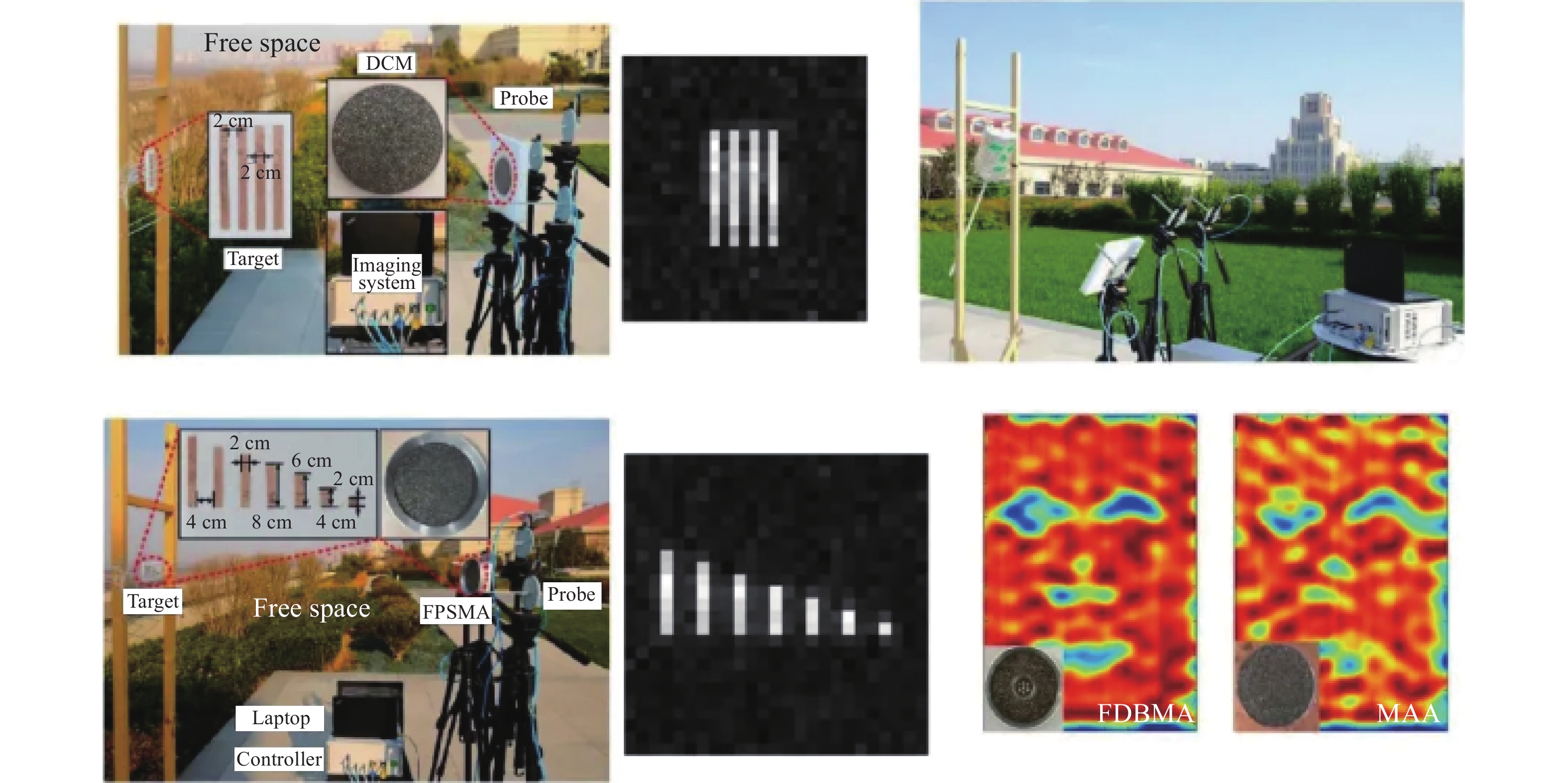
2015年,国防科技大学研制成功X波段宽带数字阵列随机波前调制成像系统,方位向空间分辨率超阵列实孔径5.6倍。2018年,开展了实际背景下地面点目标前视成像实验,如图12所示,成像距离345 m,成像分辨率超阵列实孔径10.7倍,并采用脉内随机频率调制实现了空中目标前视快拍成像,理论上单个脉冲即可实现成像,成像帧率比传统微波成像技术提高一个数量级以上。2021年,研制成功W波段波前调制成像系统,采用随机频率调制实现了实际背景下车辆目标的前视、凝视成像,成像距离100 m,成像角分辨率优于0.3°,实际目标成像分辨率超阵列实孔径10倍以上,如图13所示。

图 12 X波段波前调制点目标成像实验
Figure 12. Wavefront modulation imaging to point-targets in X band
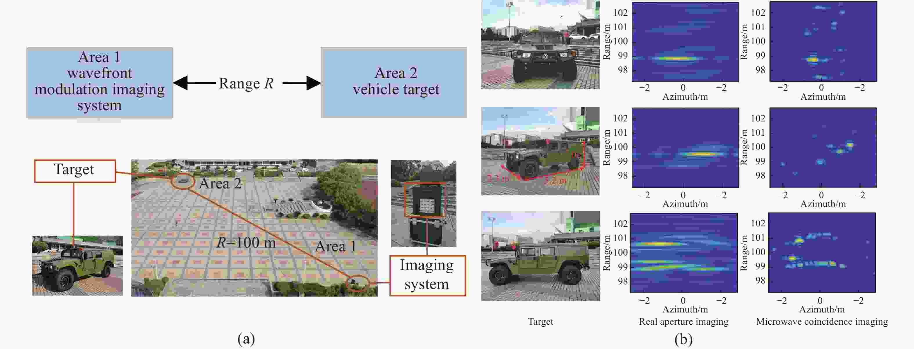
图 13 W波段波前调制车辆目标成像实验。(a) 实验场景; (b) 目标与成像结果
Figure 13. Wavefront modulation imaging to a vehicle target in W band. (a) Imaging scene; (b) Target and imaging results
-
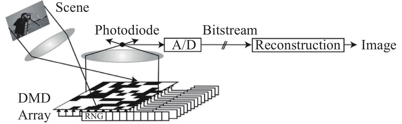
孔径编码成像起源于光学成像,主要通过对光学孔径的控制实现光瞳函数的编码,从而改善光学成像系统的传递函数,提高成像质量。2006年,Rice大学设计了光学频段单像素相机[64],系统核心部件是一块数字微镜设备(Digital micro-mirror device, DMD),DMD阵列包含数百万个微镜阵元,每个阵元通过偏转独立控制光线通断,随机组合阵元状态即可实现对光学图像的一次编码调制。DMD阵列前后各有一个透镜,光路最末端的单像素探测器检测到编码后的光强信息,结合DMD的编码模式可对原始光学图像进行解码重构,如图14所示。单像素相机采用DMD阵列代替了传统的CCD和CMOS,减少了数据存储,相比于传统光学成像更容易以低成本实现高分辨率。
2013年,杜克大学提出超材料孔径编码成像方法[65],将在接收端编码调制的单像素成像,扩展到发射端编码调制,实现主动式孔径编码成像,如图15所示。不同频率的微波信号通过超材料编码天线后在空间形成丰富的辐射模式,这些辐射模式相互正交,从而保证目标图像能够重构,其成像原理与微波关联成像是一致的。

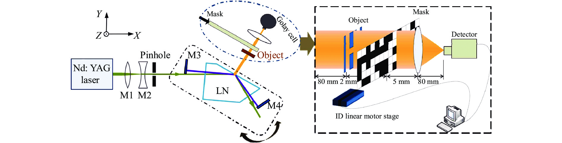
近年来,孔径编码成像逐步从光学、微波延伸至太赫兹频段,促进不同频段成像技术的发展与应用研究。2016年,天津大学与第三军医大学使用具有特定振幅编码方案的金属掩模板对太赫兹波束(0.5~2.7 THz)进行调制,金属掩模板由机械导轨驱动在光路中移动,实现编码方案的时序改变,再结合压缩感知方法,实现对特定目标的单像素太赫兹主动成像[66],如图16所示。国防科技大学在太赫兹超材料孔径编码成像原理、成像模型、编码策略以及准光系统设计等方面开展了研究[67],提出基于深度学习的太赫兹孔径编码成像算法[68-69]与基于非相干阵列探测的无相位太赫兹孔径编码成像方案[70],通过三维成像仿真[71]与一维成像实验验证了模型与算法的有效性。
-
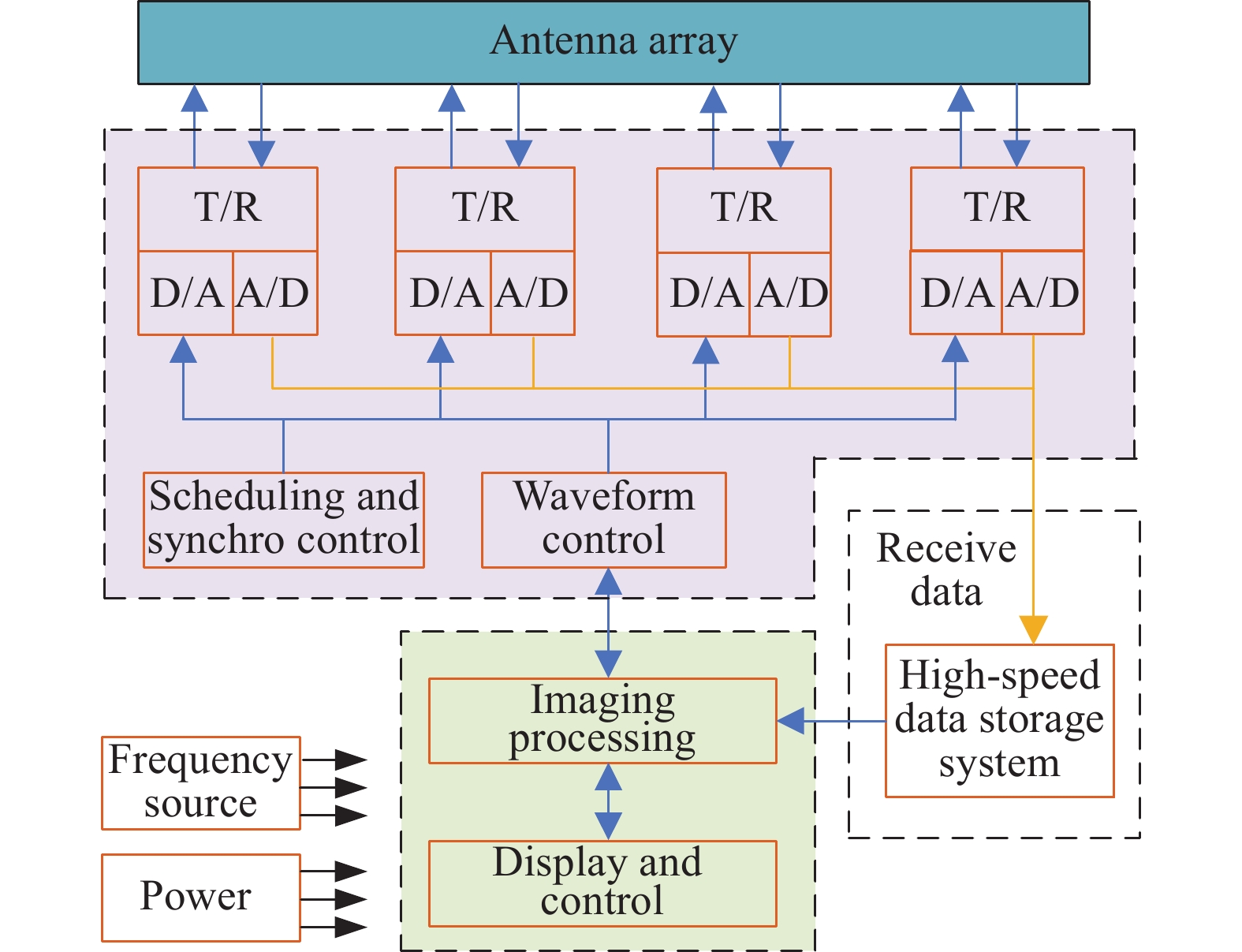
根据微波关联成像原理,成像系统的核心是通过对系统波形参数的控制产生具有时变和空变特性的辐射场。数字阵列能够对每个发射单元信号幅度、频率、相位等参数进行灵活调制,各阵元发射信号在空域叠加形成特定分布的辐射场,从而满足关联成像要求,是一种相对成熟且应用广泛的系统实现方案,随机辐射关联成像和波前调制关联成像等体制均可由数字阵列实现。数字阵列关联成像系统结构如图17所示[15],基本结构通常由天线阵列、数字发射/接收(T/R)组件、频率源、波形控制器、数据传输与存储器、成像处理器等组成。系统实现技术包括波形参数快速调制、波形精确产生与辐射场高精度预置、各通道高精度同步、通道幅相响应校准技术等。
-
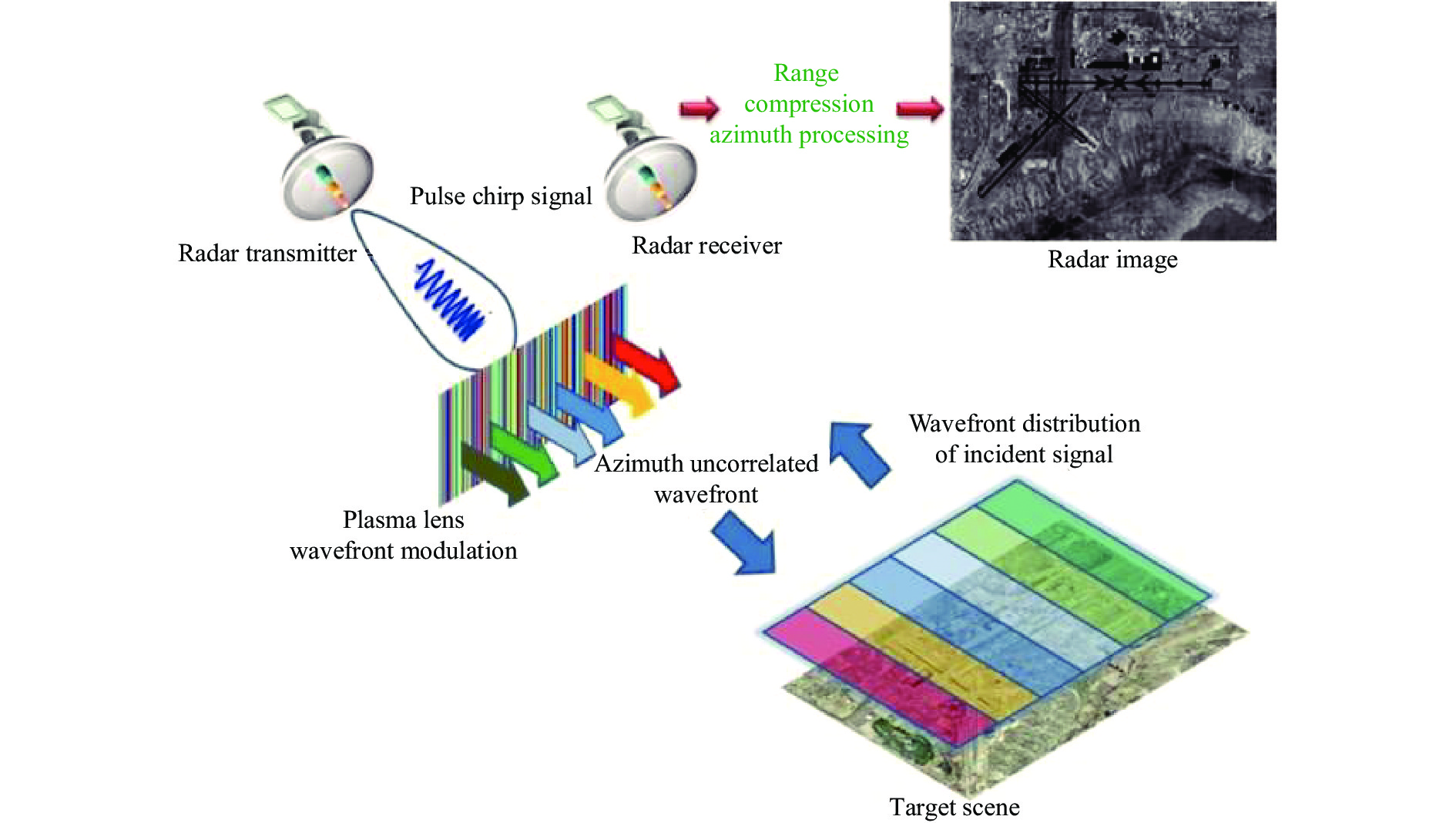
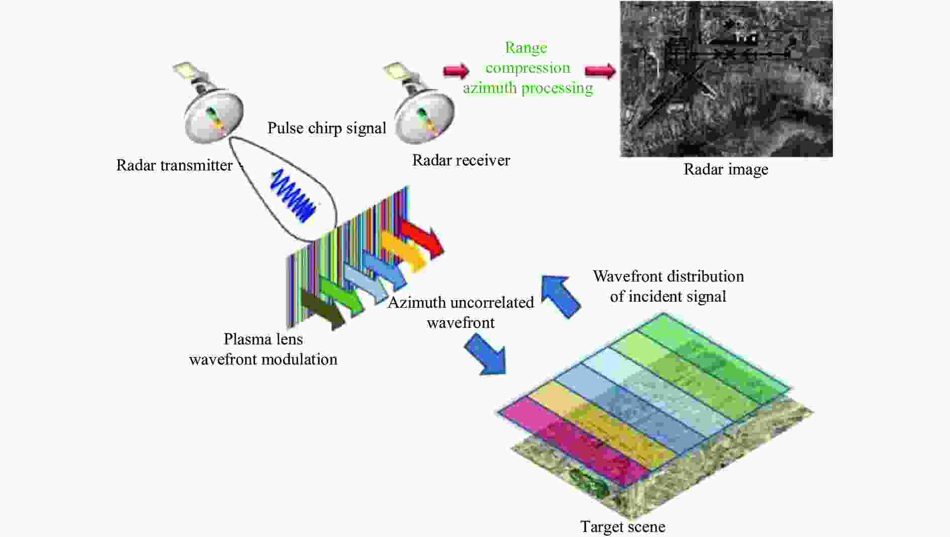
与数字阵列关联成像系统方案不同,上海交通大学利用等离子体透镜实现随机波前调制,并结合距离向脉冲压缩实现微波凝视关联成像[72],成像系统示意图如图18所示。该方法降低了辐射场观测矩阵的规模,有助于解决大场景辐射场计算复杂性难题。
-
电磁超材料由具有特殊电磁属性的人造单元结构按照一定的排列方式组成二维平面结构,其微结构与电磁波的相互作用可产生丰富的电磁响应特性,能够实现对电磁波幅度、相位等参量的自由调控,为实现微波关联成像提供了灵活的硬件基础。
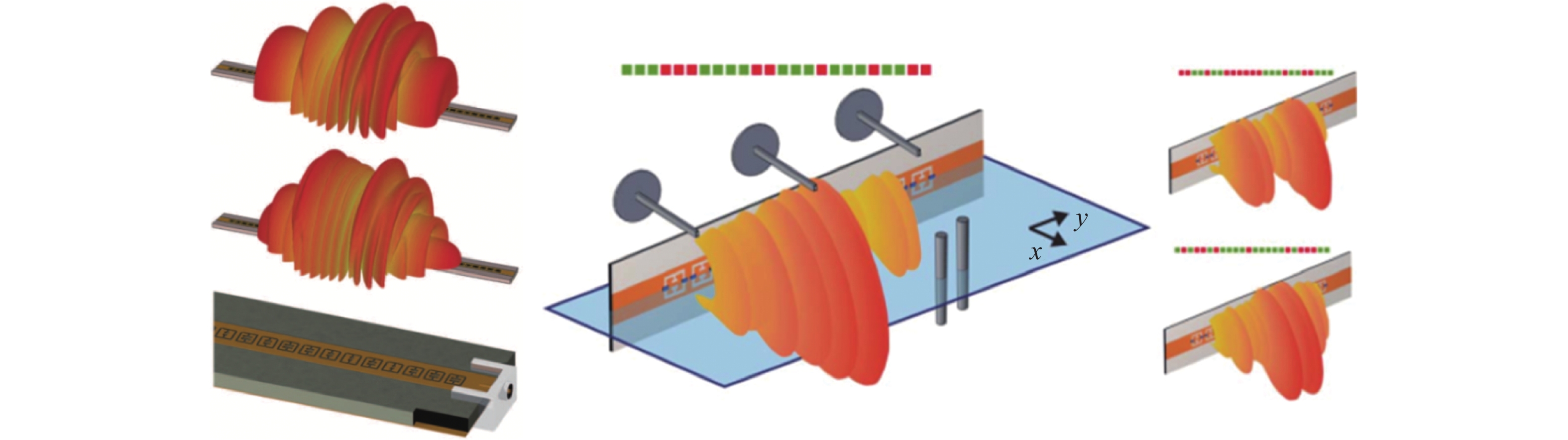
2013年,杜克大学研究了频率选择孔径编码天线特性及其在微波成像中的应用[73-74],研制了一维孔径编码天线,天线工作频段为18~26 GHz,如图19所示。在超材料表面随机排布谐振频率不同的谐振单元,激励源在天线工作带宽内进行扫频,依次激励具有不同谐振频率的谐振单元有效辐射,使得辐射方向图动态改变,产生出不同辐射模式的探测信号,从而在空间形成幅度、相位随机分布的辐射场,通过压缩感知重构目标图像[73]。2014年该团队设计了二维超材料扫频编码天线,天线工作频段为17.5~26.5 GHz,并实现了三维目标重构[74], 如图20所示 。


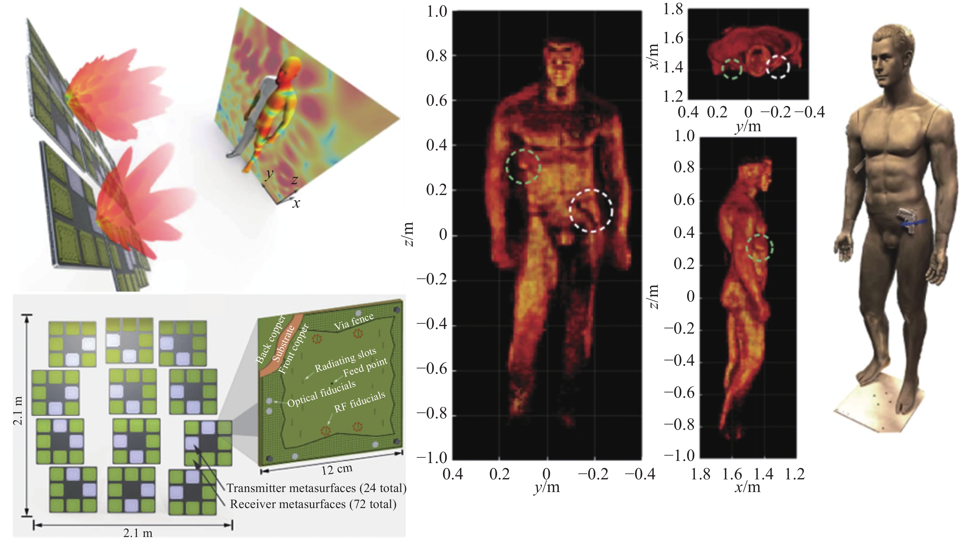
2017年,杜克大学采用12块超材料板放置于2.1 m×2.1 m的平面上,每个超材料板包含2个发射模块和6个接收模块,工作频率范围为17.5~26.5 GHz。通过超材料板位置及频率的扫描控制形成时变和空变的随机辐射模式,实现了人体目标三维成像[75],如图21所示。此外,该团队还利用超材料天线所形成的多样性辐射方向图以及天线本身运动所形成的合成孔径实现了条带式扫描合成孔径成像[76]及三维成像[77]。
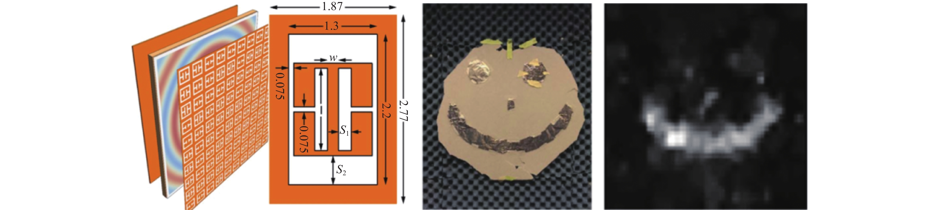
国内超材料孔径编码成像研究发展迅速。东南大学提出了基于信息超材料的孔径编码成像方法[78-79],分别于2015年和2016年,采用反射式[80]和透射式[81]可编程超材料,通过相位调制实现了单频单像素孔径编码成像。其中,透射式编码超材料采用2-bit调制,编码模式由FPGA调控,成像系统采用9.2 GHz单频信号,通过相位编码获得不同辐射模式,实现了铝箔目标成像,如图22所示。
西安交通大学提出基于电磁超表面的微波关联成像技术[82-83],在微波聚束随机辐射源设计与高效率成像算法方面开展了创新研究,研制了超表面聚束宽带随机辐射天线。利用有限孔径随机辐射源产生的辐射场空间关联特征,提出聚焦区域约束下的快速关联成像方法,在保证成像质量的前提下提高了成像速率,如图23所示。
国防科技大学针对低信噪比成像问题,提出了频域孔径编码压缩成像方法[84-85],在频域构造辐射场参考矩阵,对回波进行距离向压缩处理,获得压缩处理增益,提升成像信噪比,扩展了成像距离,实现了孔径编码三维成像。2021年,构建了Ka频段孔径编码成像系统,对金属目标模型成像,分辨率2.5 cm,超阵列实孔径约7倍,如图24所示。

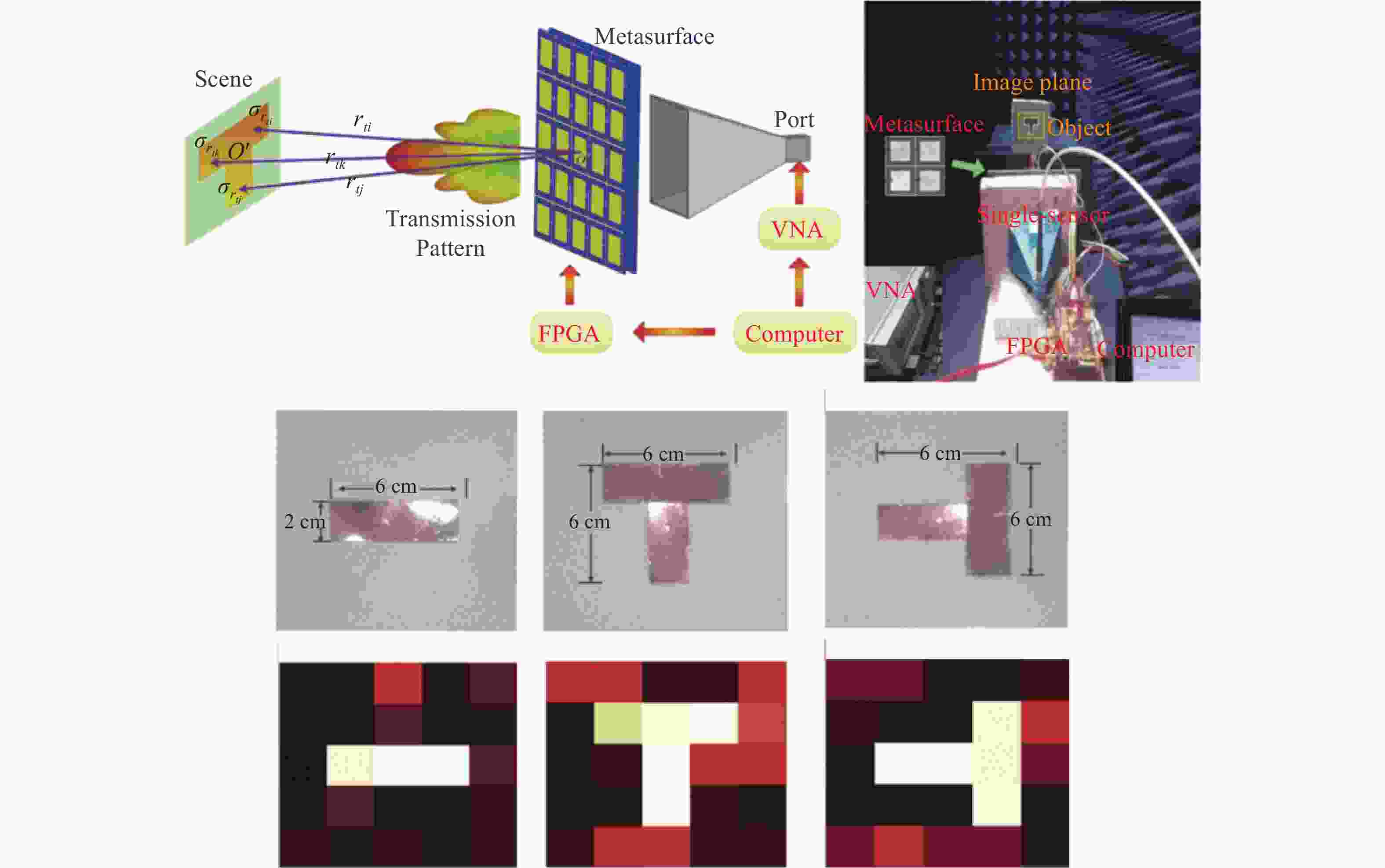


图 24 Ka频段超材料孔径编码成像实验。(a) 实验场景与成像系统;(b) 目标模型;(c) 正则化方法成像结果;(d) 稀疏贝叶斯算法成像结果
Figure 24. Coded-aperture imaging experiment in Ka band. (a) Experiment scene and imaging system; (b) Target model; (c) Imaging result of TRM algorithm; (d) Imaging result of SBL algorithm
目前,国内外已对超材料孔径编码成像技术开展了广泛研究,调制方式越来越灵活,成像维度从二维向三维扩展,有望在安检成像等领域获得应用。
-
微波关联成像作为近年来发展起来的一种新型成像技术,在成像理论以及实验验证等方面均取得了较大研究进展。文中介绍了微波关联成像的技术起源,从成像原理、成像方法、成像系统等三个方面梳理和总结了微波关联成像的研究现状及主要进展。目前,微波关联成像正朝着更高分辨率、更远成像距离、更强稳健性等方向不断发展。然而,作为一种新的成像技术,微波关联成像从理论研究到实际应用还存在诸多科学与技术问题需要突破和解决,其未来发展趋势主要体现在以下四个方面:
(1)不同调制方式的成像机理与成像方法。随着电磁波调控技术的发展,微波关联成像的信号调制方式呈现出随机辐射场、电磁涡旋波前等各种形式。其中,随机辐射场利用电磁信号在空间上的随机涨落,形成差异性激励,获得空间分辨信息;电磁涡旋利用方位维周期性的相位梯度,形成方位维分辨能力。理论上通过对电磁信号多维参量的编码设计,可以产生新的调制模式,衍生出新的成像方法。然而,无论哪种调制方式,其共同特点都要具备时变和空变的辐射特性。其中,空变特性决定固有的成像分辨能力,时变特性决定了成像重构效率,二者共同构成了成像重构的基本条件,而成像方法又会影响成像质量与成像性能。各种调制方式下的成像分辨机理与成像方法有联系也有区别,是微波关联成像理论研究的重点,包括辐射场与目标相互作用机理及目标散射特性、各种形式成像模型的演化、成像重构条件、稳健重构算法等。另外,随着计算资源和计算能力的提升,计算成像理论的发展也将促进微波关联成像方法研究。
(2)远距离高分辨成像性能增强技术。微波关联成像通过电磁信号调制形成具有空间差异性的辐射场获得方位向空间分辨能力的提升。然而,空域非相干特性造成信号增益降低,相比传统成像技术,信号发射与接收增益及处理增益均有损失,需研究远距离低信噪比成像技术。另外,由于电磁波传播特性,辐射场空间差异性随距离减弱,在获得角度超分辨率的同时,进一步提高空间分辨率也是实际应用中需要解决的重要问题。通过将距离-方位解耦、距离向脉冲压缩结合方位向高分辨处理,以及辐射场聚束设计等,可以在一定程度上提升远距离高分辨成像性能。
(3)高效稳定的辐射源与系统构建技术。辐射场的快速调制与精确预置是微波关联成像的基础,高稳定度辐射源是其中的关键。深入研究数字阵列、等离子体透镜、超材料与超表面等调制技术,探索新型微波调制器件及系统构建技术,发展微波调控新手段与成像系统新体制,研究系统误差自适应校正与补偿技术,以及辐射场优化与特性增强技术,生成灵活调制的微波辐射场,以满足稳健成像应用需求。
(4)复杂环境实际目标成像应用关键技术。实际应用需求是促进成像技术发展的驱动力。相比传统成像技术,微波关联成像具有凝视、前视、快拍成像等优势,有望与传统成像技术形成互补。结合应用场景分析各种边界条件对成像性能的约束,充分认识和掌握微波关联成像的性能优势与不足,取长补短,面向无人系统目标及环境自主感知、重点区域凝视观测、要地防御、目标识别、安检安防等领域的应用前景,研究并突破其中的关键技术问题,形成典型应用,是微波关联成像未来发展的重点。
Progress and prospect of microwave coincidence imaging(Invited)
-
摘要: 微波关联成像起源于光学强度关联成像,通过对电磁波的调控形成空变和时变的辐射模式,突破天线孔径对成像分辨率的限制,具有前视、凝视、快拍成像等优势,在重点区域凝视观测、无人系统自主感知、安检安防等领域具有广阔的应用前景。文中简述了微波关联成像的技术起源,从成像原理、成像方法、成像系统等三个方面,总结了微波关联成像的研究现状与主要进展。通过对成像原理的剖析,阐明关联成像的基本条件与成像分辨率的影响因素;通过对成像方法的梳理,分析微波关联成像与光学关联成像以及传统微波成像方法之间的区别与联系;通过对成像系统的介绍,比较随机辐射、波前调制、孔径编码等多种成像体制的特点与差异,厘清技术发展脉络。最后,总结并展望了微波关联成像的未来发展趋势。Abstract: Originated from the optical intensity ghost imaging, microwave coincidence imaging breaks through the limitation of antenna aperture on imaging resolution by space and time-varying radiation mode through the modulation of electromagnetic waves. It has the advantages of forward-looking, staring and fast-shooting imaging, and has broad application prospects in the fields of staring observation in key areas, autonomous sensing of unmanned systems, security inspection and security protection and so on. The technical origin of microwave coincidence imaging was briefly described, and its current research status and main progress from three aspects including the imaging principle, imaging methods and imaging systems were summarized. Through the analysis of the imaging principle, the basic conditions for coincidence imaging and the influencing factors of imaging resolution were clarified. Through the review of imaging methods, the differences and relationships among microwave coincidence imaging, optical ghost imaging and conventional microwave imaging methods were analyzed. Through the introduction of imaging systems, the features and differences among various systems such as random radiation, wavefront modulation and aperture encoding were compared, which made the development of microwave coincidence imaging easier to perceive. Finally, the future development trend of microwave coincidence imaging was summarized and prospected.
-
图 3 微波关联成像分辨率表征[15]。(a) 传统成像相干发射情形;(b) 关联成像非相干发射情形;(c) 传统成像空间相关函数;(d) 关联成像空间相关函数
Figure 3. Resolution analysis of microwave coincidence imaging[15]. (a) Coherent transmissions of conventional imaging; (b) Incoherent transmissions of coincidence imaging; (c) Spatial correlation function of conventional imaging; (d) Spatial correlation function of coincidence imaging
图 4 不同发射波形的空间相关函数[9]。(a)~(b) 随机调频波形辐射场和空间相关函数;(c)~(d) 随机调幅波形辐射场和空间相关函数;(e)~(f) 随机调相波形辐射场和空间相关函数
Figure 4. Spatial correlation functions of transmitted waveforms[9]. (a)-(b) Radiation field and spatial correlation function of random frequency modulation waveform; (c)-(d) Radiation field and spatial correlation function of random amplitude modulation waveform; (e)-(f) Radiation field and spatial correlation function of random phase modulation waveform
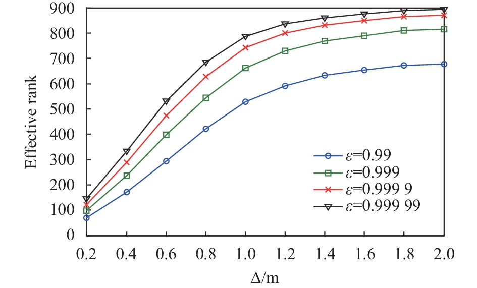
图 6 各种微波关联成像算法结果对比。(a) 目标场景;(b) 相关法;(c) 最小二乘法;(d) Tikhonov正则化方法;(e) SBL
Figure 6. Comparison of various algorithms of microwave coincidence imaging. (a) Target scene; (b) Correlation; (c) Least square; (d) Tikhonov regularization; (e) SBL
图 11 典型波前调制形式。(a) 随机波前;(b) 涡旋波前
Figure 11. Typical wavefront modulation forms. (a) Random wavefront; (b) Vortex wavefront
图 12 X波段波前调制点目标成像实验
Figure 12. Wavefront modulation imaging to point-targets in X band
图 13 W波段波前调制车辆目标成像实验。(a) 实验场景; (b) 目标与成像结果
Figure 13. Wavefront modulation imaging to a vehicle target in W band. (a) Imaging scene; (b) Target and imaging results


-
[1] Ausherman D A, Kozma A, Walker J L, et al. Developments in radar imaging [J]. IEEE Transactions on Aerospace and Electronic Systems, 1984, 20(4): 363-400. [2] Nan Y J, Huang X J, Guo Y J. Generalized continuous wave synthetic aperture radar for high resolution and wide swath remote sensing [J]. IEEE Transactions on Geoscience and Remote Sensing, 2018, 56(12): 7217-7229. doi: 10.1109/TGRS.2018.2849382 [3] Zhang L, Qiao Z J, Xing M D, et al. High-resolution ISAR imaging by exploiting sparse apertures [J]. IEEE Transactions on Antennas and Propagation, 2012, 60(2): 997-1008. doi: 10.1109/TAP.2011.2173130 [4] Yang J Y. Multi-directional evolution trend and law analysis of radar ground imaging technology [J]. Journal of Radars, 2019, 8(6): 669-693. (in Chinese) [5] Liu W T, Sun S, Hu H K, et al. Progress and prospect for ghost imaging of moving objects [J]. Laser and Optoelectronics Progress, 2021, 58(10): 3-16. (in Chinese) [6] Guo Y Y, Wang D J, He X Z, et al. Super-resolution imaging method based on random radiation radar array[C]//2012 IEEE International Conference on Imaging Systems and Techniques Proceedings, Manchester, 2012: 1-6. [7] Guo Y Y, He X Z, Wang D J. A novel super-resolution imaging method based on stochastic radiation radar array [J]. Measurement Science and Technology, 2013, 24(7): 074013. doi: 10.1088/0957-0233/24/7/074013 [8] He X Z. The information processing methods and simulations in microwave staring correlated imaging[D]. Hefei: University of Science and Technology of China, 2013. (in Chinese) [9] Li D Z. Radar coincidence imaging technique research[D]. Changsha: National University of Defense Technology, 2014. (in Chinese) [10] Shao Z L. Design on spatial-temporal random radiation field for compressed sensing based microwave imaging radar[D]. Xi’an: Xidian University, 2014. (in Chinese) [11] Xu R. Study on new systems and techniques for improving radar imaging performances[D]. Xi’an: Xidian University, 2015. (in Chinese) [12] Chen J P, Zhu W G, Zhang G. A new method of microwave relating imaging [J]. Journal of Naval Aeronautical and Astronautical University, 2012, 27(2): 196-198. (in Chinese) doi: 10.3969/j.issn.1673-1522.2012.02.016 [13] Shao P, Xu R, Li H L, et al. The research on bjorck-schmidt orthogonalization for microwave staring imaging [J]. Journal of Signal Processing, 2014, 30(4): 450-456. (in Chinese) [14] Zhu S T, Zhang A X, Xu Z, et al. Radar coincidence imaging with random microwave source [J]. IEEE Antennas Wireless Propagation Letters, 2015, 14: 1239-1242. doi: 10.1109/LAWP.2015.2399977 [15] Cheng Y Q, Zhou X L, Xu X W, et al. Radar coincidence imaging with stochastic frequency modulated array [J]. IEEE Journal of Selected Topics in Signal Processing, 2016, 8(5): 513-524. [16] Xu X W. Research on radar coincidence imaging with array position error[D]. Changsha: National University of Defense Technology, 2015. (in Chinese) [17] Zhou X L. Theory and methods of sparsity-based microwave coincidence imaging[D]. Changsha: National University of Defense Technology, 2017. (in Chinese) [18] Zha G F. Microwave coincidence imaging technique research for moving target[D]. Changsha: National University of Defense Technology, 2016. (in Chinese) [19] Zhu S T, He Y C, Chen X M, et al. Resolution threshold analysis of the microwave radar coincidence imaging [J]. IEEE Transactions on Geoscience and Remote Sensing, 2020, 58(3): 2232-2243. doi: 10.1109/TGRS.2019.2955789 [20] Wang T Y. Research on distributed radar sparse imaging technologies[D]. Hefei: University of Science and Technology of China, 2015. (in Chinese) [21] Kay S M. Fundamentals of Statistical Signal Processing: Estimation Theory[M]. Englewood: Prentice Hall, 1993. [22] Albert A. Regress and the Moore-Penrose Pseudoinverse[M]. New York: Academic Press, 1972. [23] Golub G H, Van Loan C F. Matrix Computations[M]. 3rd ed. Baltimore: Johns Hopkins University Press, 1996. [24] Yang J G. Research on sparsity-driven regularization radar imaging theory and method[D]. Changsha: National University of Defense Technology, 2014. (in Chinese) [25] Phillips D L. A technique for the numerical solution of certain integral equations of the first kind [J]. Journal of the Association for Computing Machinery, 1962, 9: 84-97. doi: 10.1145/321105.321114 [26] Tikhonov A N. Solution of incorrectly formulated problems and the regularization method [J]. Soviet Mathematics-Doklady, 1963, 4: 1035-1038. [27] Potter L C, Chiang D, Carriere R, et al. A GTD-based parametric model for radar scattering [J]. IEEE Transactions on Antennas Propagation, 1995, 32(10): 1058-1067. [28] Baraniuk R G. Compressive sensing [J]. IEEE Signal Processing Magazine, 2007, 24(4): 118-121. doi: 10.1109/MSP.2007.4286571 [29] Donoho D L. For most large underdetermined systems of linear equations, the minimal L1 norm solution is also the sparsest solution [J]. Communications on Pure and Applied Mathematics, 2006, 59(6): 797-829. doi: 10.1002/cpa.20132 [30] Candès E J, Wakin M B. An introduction to compressive sampling: a sensing/sampling paradigm that goes against the common knowledge in data acquisition [J]. IEEE Signal Processing Magazine, 2008, 25(2): 21-30. doi: 10.1109/MSP.2007.914731 [31] Chen S, Donoho D, Saunders M. Atomic decomposition by basis pursuit [J]. SIAM Review, 2001, 43(1): 129-159. doi: 10.1137/S003614450037906X [32] Tropp J A, Gilbert A C. Signal recovery from random measurements via orthogonal matching pursuit [J]. IEEE Transactions on Information Theory, 2007, 53(12): 4655-4666. doi: 10.1109/TIT.2007.909108 [33] Wipf D P, Rao B D. Sparse Bayesian learning for basis selection [J]. IEEE Transactions on Signal Processing, 2004, 52(8): 2153-2164. doi: 10.1109/TSP.2004.831016 [34] Guo Y, Ma Y, Wang D. A novel microwave staring imaging method based on short-time integral stochastic radiation fields[C]//2013 IEEE International Conference on Imaging Systems and Techniques, 2013: 425-430. [35] Ma Y P. Preliminary research on microwave staring correlated imaging based on temporal-spatial stochastic radiation fields[D]. Hefei: University of Science and Technology of China, 2013. (in Chinese) [36] Xu X W, Cheng Y Q, Qin Y L, et al. Analysis of array position error in radar coincidence imaging [J]. Modern Radar, 2016, 38(3): 32-37. (in Chinese) [37] Xu X W, Zhou X L, Cheng Y Q, et al. Radar coincidence imaging with array position error[C]//2015 IEEE International Conference on Signal Processing, Communications and Computing (ICSPCC 2015), 2015: 119-122. [38] Yi M L. Study on compressed sensing algorithm for microwave staring imaging[D]. Xi’an: Xidian University, 2014. (in Chinese) [39] Zhou X, Wang H, Cheng Y, et al. Sparse auto-calibration for radar coincidence imaging with gain-phase error [J]. Sensors, 2015, 15: 27611-27624. doi: 10.3390/s151127611 [40] Zhou X, Wang H, Cheng Y, et al. Radar coincidence imaging with phase error using Bayesian hierarchical prior modeling [J]. Journal of Electronic Imaging, 2016, 25(1): 013018. doi: 10.1117/1.JEI.25.1.013018 [41] Zhou X, Wang H, Cheng Y, et al. An ExCoV-based method for joint radar coincidence imaging and gain-phase error calibration [J]. Mathematical Problems in Engineering, 2016, 8(5): 513-524. [42] Zheng Y. Array self-calibration for MIMO radar with gain-phase error[D]. Xi’an: Xidian University, 2015. (in Chinese) [43] Zhou X, Wang H, Cheng Y, et al. Off-grid radar coincidence imaging based on block sparse Bayesian learning[C]//2015 IEEE Workshop on Signal Processing Systems (SiPS), 2015: 440-443. [44] Li D, Li X, Cheng Y, et al. Radar coincidence imaging under grid mismatch [J]. ISRN Signal Processing, 2014, 987803: 1-8. [45] Luo C S. Research on microwave correlated sparse imaging of moving target[D]. Hefei: University of Science and Technology of China, 2016. (in Chinese) [46] Wang G C. Research on microwave staring correlated imaging of low-rank and large scene[D]. Hefei: University of Science and Technology of China, 2018. (in Chinese) [47] Meng Q Q. The research on information processing in high resolution microwave staring correlated imaging[D]. Hefei: University of Science and Technology of China, 2016. (in Chinese) [48] Cao K C, Cheng Y Q, Liu K, et al. Off-grid microwave coincidence imaging based on directional grid fission [J]. IEEE Antennas Wireless Propagation Letters, 2020, 19(12): 2497-2501. doi: 10.1109/LAWP.2020.3037100 [49] Cao K C, Cheng Y Q, Liu K, et al. Reweighted-dynamic-grid-based microwave coincidence imaging with grid mismatch[J/OL]. IEEE Transactions on Geoscience and Remote Sensing(2021-06-15)https://ieeexplore.ieee.org/document/9455128/authors#authors. [50] Zhang H L. Research on sparse reconstruction technology for microwave staring correlated imaging of moving target[D]. Hefei: University of Science and Technology of China, 2015. (in Chinese) [51] Li D Z, Li X, Cheng Y Q, et al. Radar coincidence imaging in the presence of target-motion-induced error [J]. Journal of Electronic Imaging, 2014, 23(2): 023014. doi: 10.1117/1.JEI.23.2.023014 [52] Li D Z, Li X, Qin Y L, et al. Radar coincidence imaging: an instantaneous imaging technique with stochastic signals [J]. IEEE Transactions on Geoscience and Remote Sensing, 2014, 52(4): 2261-2277. doi: 10.1109/TGRS.2013.2258929 [53] Yu H. Research on sparse imaging algorithms for correlated imaging systems[D]. Hefei: University of Science and Technology of China, 2014. (in Chinese) [54] Yang H T, Wang K Z, Yuan B, et al. Microwave staring imaging based on range pulse compression and azimuth wavefront modulation[C]//10th European Conference on Synthetic Aperture Radar (EUSAR 2014), 2014: 1-4. [55] Yuan Y, Li C R, Li X H, et al. Sensitivity analysis on radiant performance of microwave intensity correlation image [J]. Remote Sensing Technology and Application, 2015, 1(30): 155-162. (in Chinese) [56] Zhou X, Wang H, Cheng Y, et al. Radar coincidence imaging for off-grid target using frequency-hopping waveforms [J]. International Journal of Antennas and Propagation, 2016, 2016: 1-16. doi: 10.1155/2016/8523143 [57] Zhou X L, Wang H Q, Cheng Y Q, et al. Radar coincidence imaging by exploiting the continuity of extended target [J]. IET Radar, Sonar & Navigation, 2017, 11(1): 60-69. [58] Zhou X, Wang H, Cheng Y, et al. Off-grid radar coincidence imaging based on variational sparse Bayesian learning [J]. Mathematical Problems in Engineering, 2016, 2016: 1782178. [59] Cao K C, Cheng Y Q, Liu K, et al. Coherent-detecting and incoherent-modulating microwave coincidence imaging with off-grid errors[J/OL]. IEEE Geoscience and Remote Sensing Letters(2021-11-13)https://ieeexplore.ieee.org/document/9612163. [60] Dai Q. Research on radar coincidence imaging technology in low SNR[D]. Changsha: National University of Defense Technology, 2014. (in Chinese) [61] Cao K C. Research on radar coincidence imaging with model mismatch[D]. Changsha: National University of Defense Technology, 2017. (in Chinese) [62] Yuan T Z. Research on radar imaging using electromagnetic vortex wave[D]. Changsha: National University of Defense Technology, 2017. (in Chinese) [63] Liu K. Study on the theory and method of electromagnetic vortex imaging[D]. Changsha: National University of Defense Technology, 2017. (in Chinese) [64] Laska J N, Wakin M B, Duarte M F, et al. A new compressive imaging camera architecture using optical-domain compression[C]//Conference on Computational Imaging IV, 2006: 606509. [65] Hunt J D. Metamaterials for computational imaging[D]. Durham: Duke University, 2013. [66] Duan P, Wang Y Y, Xu D G, et al. Single pixel imaging with tunable terahertz parametric oscillator [J]. Applied Optics, 2016, 55(13): 3670-3675. doi: 10.1364/AO.55.003670 [67] Chen S, Luo C G, Deng B, et al. Study on coding strategies for radar coded-aperture imaging in terahertz band [J]. Journal of Electronic Imaging, 2017, 26(5): 053022. [68] Gan F J, Luo C G, Liu X Y, et al. Fast terahertz coded-aperture imaging based on convolutional neural network [J]. Applied Sciences-Basel, 2020, 10(8): 2661. doi: 10.3390/app10082661 [69] Gan F J, Yuan Z Y, Luo C G, et al. Phaseless terahertz coded-aperture imaging based on deep generative neural network [J]. Remote Sensing, 2021, 13(671): 1-15. [70] Liu X Y, Wang H Q, Luo C G, et al. Terahertz coded-aperture imaging for moving targets based on incoherent detection array [J]. Applied Optics, 2021, 60(23): 6809-6817. doi: 10.1364/AO.428457 [71] Luo C G, Deng B, Wang H Q, et al. High-resolution terahertz coded-aperture imaging for near-field three-dimensional target [J]. Applied Optics, 2019, 58(12): 3293-3300. doi: 10.1364/AO.58.003293 [72] Yang H T, Zhang L J, Gao Y S, et al. Azimuth wavefront modulation using plasma lens array for microwave staring imaging[C]//IEEE Geoscience and Remote Sensing Symposium, 2015: 4276-4279. [73] Sleasman T, Boyarsk M, Imani M F, et al. Design considerations for a dynamic metamaterial aperture for computational imaging at microwave frequencies [J]. Journal of the Optical Society of America B, 2016, 33(6): 1098-1111. doi: 10.1364/JOSAB.33.001098 [74] Hunt J, Gollub J, Driscoll T, et al. Metamaterial microwave holographic imaging system [J]. Journal of the Optical Society of America A, 2014, 31(10): 2109-2119. doi: 10.1364/JOSAA.31.002109 [75] Gollub J N, Yurduseven O, Trofatter K P, et al. Large metasurface aperture for millimeter wave computational imaging at the human-scale [J]. Scientific Reports, 2017, 7: 42650. doi: 10.1038/srep42650 [76] Andreas P, Claire M W, Smith D R, et al. Enhanced resolution stripmap mode using dynamic metasurface antennas [J]. IEEE Transactions on Geoscience and Remote Sensing, 2017, 55(7): 3764-3772. doi: 10.1109/TGRS.2017.2679438 [77] Sleasman T, Boyarsky M, Pulido-Mancera L, et al. Experimental synthetic aperture radar with dynamic metasurfaces [J]. IEEE Transactions on Antennas and Propagation, 2017, 65(12): 6864-6877. doi: 10.1109/TAP.2017.2758797 [78] Cui T J, Wu R Y, Wu W, et al. Large-scale transmission-type multifunctional anisotropic coding metasurfaces in millimeter-wave frequencies [J]. Journal of Physics D:Applied Physics, 2017, 50(40): 404002. doi: 10.1088/1361-6463/aa85bd [79] Liu S, Cui T J. Concepts, working principles, and applications of coding and programmable metamaterials [J]. Advanced Optical Materials, 2017, 5(22): 1700624. doi: 10.1002/adom.201700624 [80] Wang L, Li L, Li Y, et al. Single-shot and single-sensor high/super-resolution microwave imaging based on metasurface [J]. Scientific Reports, 2016, 6: 26959. doi: 10.1038/srep26959 [81] Li Y B, Li L L, Xu B B, et al. Transmission-type 2-bit programmable metasurface for single-sensor and single-frequency microwave imaging [J]. Scientific Reports, 2016, 6: 23731. doi: 10.1038/srep23731 [82] Zhao M R, Zhu S T, Huang H L, et al. Frequency-polarization-sensitive metasurface antenna for coincidence imaging [J]. IEEE Antennas and Wireless Propagation Letters, 2021, 20(7): 1274-1278. doi: 10.1109/LAWP.2021.3077556 [83] Zhao M R, Zhu S T, Huang H L, et al. Frequency-diverse metamaterial cavity antenna for coincidence imaging [J]. IEEE Antennas and Wireless Propagation Letters, 2021, 20(6): 1103-1107. doi: 10.1109/LAWP.2021.3073679 [84] Chen S. Research on technology of three-dimensional terahertz coded-aperture imaging[D]. Changsha: National University of Defense Technology, 2018. (in Chinese) [85] Luo Z L. Research on coded aperture imaging based on programmable metasurface[D]. Changsha: National University of Defense Technology, 2018. (in Chinese) -

 点击查看大图
计量
- 文章访问数: 646
- HTML全文浏览量: 128
- PDF下载量: 133
- 被引次数: 0


