


 /nm
/nm /m
/m /μJ
/μJ /ns
/ns


-
2020年9月,在第七十五届联合国大会上,我国明确提出二氧化碳排放力争于2030年前达到峰值,于2060年前实现碳中和[1]。全球自然生态系统通过光合作用捕获的碳(称为“生物碳”) 55%由海洋生物捕获[2],其中颗粒有机碳(POC)是碳在海洋中的重要存在形式。因此,对海洋中POC含量的探测,将对海洋碳汇能力的评估起到重要作用。
统计显示截至2019年,海洋观测数据一半的贡献来自于卫星遥感,该技术不但可以实现大面积的同步观测,还能满足长时间动态观测的需求[3]。但这种方法的缺点在于获取海洋剖面信息的能力有限,而激光雷达是目前已知有望实现海洋真光层剖面结构信息探测的技术手段[4]。
高光谱分辨率激光雷达(High Spectral Resolution Lidar, HSRL)是一种利用回波信号后向散射谱中粒子散射和分子散射的谱宽量级不同,使用窄带滤波器(或滤光器)实现光谱分离的激光雷达。HSRL技术突破了求解标准后向散射激光雷达方程存在的“一个方程,两个未知数”问题,无需假设激光雷达比便可高精度求解[5]。
为此,国内外的研究机构利用HSRL技术对海洋剖面信息进行了广泛研究。2017年,Schulien等人利用美国国家航天局(NASA)的HSRL进行了船载和机载光学研究,并对同时采集的数据进行比较和反演得到了浮游植物碳和净初级生产力的垂直分布[6]。其在2020年的最新研究表明,通过HSRL技术可以揭示混合层浮游植物的垂直和水平分布的复杂结构[7]。
2017年,浙江大学与自然资源部第二海洋研究所共同研制的532 nm弹性散射激光雷达并于黄海进行海试,结果表明海洋激光雷达能够准确地探测上层海水的剖面信息[8-9]。2018年,中国科学院上海光学精密机械研究所和自然资源部第二海洋研究所研制的双通道机载激光雷达Mapper5000在中国南海三亚湾海区机载平台上进行了三次试验,成功实现了水深50 m内的浮游生物层探测,并得到了三亚湾海域浮游生物次表层的空间分布和季节变化[10-11]。
激光雷达系统的研制是一项耗时且庞杂的工程,因此有必要在研制初期对系统参数进行仿真分析和优化,以确保激光雷达系统的可行性和可用性。2020年,Liu Qun等人利用中分辨率成像光谱仪(MODIS)的海洋光学特性数据,模拟计算了激光雷达在全球最大穿透深度的分布和相应的最佳波段[12],为未来星载平台激光雷达系统参数设计提供了一定参考。
不同搭载平台的激光雷达系统由于工作环境的不同,相应参数设置和性能也有所不同。而目前有关船载、机载激光雷达系统参数仿真的研究较少。为此,文中利用中国海洋大学的星载海洋激光雷达仿真系统获得海域的水体参数[13],估算了机载海洋激光雷达系统在不同海域的最佳穿透深度分布;针对船载和机载两种搭载平台,利用HSRL技术实现海洋POC探测的最佳工作波长,为实际海洋POC探测系统的设计提供参考。
-
激光雷达探测系统的原理是向海洋发射激光脉冲,并使用单光子探测器收集散射光,经过数据反演得到海洋剖面信息。因此,仿真核心即依据激光雷达方程进行海洋剖面回波光电子数的模拟。
用激光雷达方程表述的水面以下垂直距离z处返回的光电子数如公式(1)所示:
$$ \begin{split} & {N}_{phoele}\left({{z}}\right)=\\ & \frac{\dfrac{E\cdot A\cdot O\cdot {T}_{0}\cdot {T}_{s}^{2}\cdot n\cdot c\cdot \Delta T\cdot \eta }{2(nH+{{z}}{)}^{2}}\beta (\pi ,{{z}})\mathit{{\rm{exp}}}[-2{\displaystyle\int }_{0}^{{{z}}}\alpha \left({{{z}}}'\right){\rm{d}}{{{z}}}']}{hv} \end{split} $$ (1) 式中:E代表激光出射单脉冲能量;A为接收望远镜有效面积;O代表雷达重叠因子;
$ {T}_{0} $ 代表发射接收系统的光学损耗;$ {T}_{s} $ 代表海气界面的透过率;n代表海水折射率;c代表光速;$ \Delta T $ 代表脉冲宽度;H代表机载平台的飞行高度;z代表在海水中的传输深度;$\;\beta (\pi ,{{z}})$ 代表z处的后向180°体散射系数;$\alpha \left({{z}}\right)$ 代表z处的光束衰减系数;η表示探测器光电转换效率。激光雷达接收到的是颗粒物和分子的后向散射光,即公式(1)中的$\beta (\pi ,{{z}})$ 可表示为:$$ \beta \left(\pi ,{{z}}\right)={\beta }_{particle}\left(\pi ,{{z}}\right)+{\beta }_{mol,ray}\left(\pi ,{{z}}\right)+{\beta }_{mol,brill}\left(\pi ,{{z}}\right) $$ (2) 式中:
$\;{\beta }_{particle}(\pi ,{{z}})$ 代表颗粒物的后向180°体散射系数,它与叶绿素浓度密切相关,可通过叶绿素浓度反演得到,POC的浓度即与该参数密切相关;$\;{\beta }_{mol,ray}(\pi ,{{z}})$ 为分子瑞利后向180°体散射系数;$\;{\beta }_{mol,brill}(\pi ,{{z}})$ 为分子布里渊后向180°体散射系数。激光雷达方程是仿真模拟的核心依据,通过分离散射光谱得到颗粒物的后向散射强度,进而可通过算法反演得到海洋POC剖面信息。
-
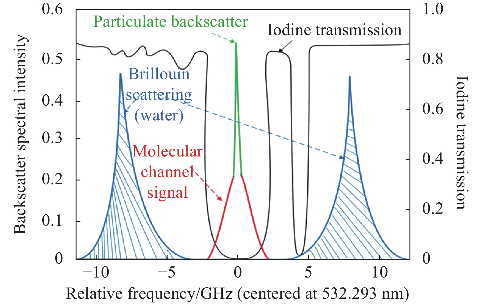
准确反演海洋POC剖面信息关键的一步是从回波信号中提取颗粒物的后向散射信号。在洁净的大洋I类水体中[14],分子散射以非弹性散射的布里渊散射为主,颗粒物散射以弹性散射的米散射为主,两者的散射谱宽度存在数量级差异。高光谱分辨率探测使用与发射激光波长相匹配的窄带滤波器实现分子散射和米散射(POC)信号的区分。碘分子吸收池结构简单,对入射角要求不高,且在532 nm附近有多条吸收线,所以成为大多数HSRL的首选滤光器。基于碘分子吸收池的光谱滤波原理如图1所示。

图 1 碘分子吸收池高光谱分辨率探测原理
Figure 1. High spectral resolution detection principle for iodine molecular absorption cells
由图1可知,当碘分子吸收线与发射激光波长相匹配时,代表POC的米散射信号可被完全吸收,代表分子散射的布里渊散射信号几乎可以完全透过,进而从光谱上实现颗粒物散射信号和分子散射信号的分离。
从激光雷达回波信号到反演POC浓度需要历经三步。第一步:从激光雷达信号反演叶绿素浓度,这一步的反演误差
${\sigma }_{{\rm{chl-a}}}=18.4{\text{%}}$ ;第二步:从叶绿素浓度反演颗粒物后向散射系数bbp模型,这一步的反演误差${\sigma }_{{\rm{bbp}}}=6{\text{%}}$ ;第三步:从颗粒物后向散射系数bbp反演POC浓度,这一步的反演误差为${\sigma }_{{\rm{POC}}}= 5.3{\text{%}}$ [8]。从激光雷达信号到POC浓度反演的三个步骤中,第一步的误差最大,这是因为激光雷达接收的光强信号是颗粒物散射和分子散射的总和,无法区分。因此,使用碘池区分激光雷达回波信号中的颗粒物回波信号强度和分子回波信号强度,可降低叶绿素浓度的反演误差,从而提升POC浓度的反演精度。
-
散射光的退偏信息是研究粒子形态的一种重要判别特征[15]。探测系统通过分偏振的方式将回波信号光分为正交探测通道和平行探测通道,以获得粒子的退偏信息,对粒子进行分类。在正交探测通道,主要响应的是非球形粒子POC散射信息;在平行通道,主要响应的是球形粒子POC和分子散射信息总和。假设POC主要近似为球形颗粒。为提取平行通道的POC信息,系统结合碘池532 nm附近吸收线设计了高光谱滤波模式,如图2所示。
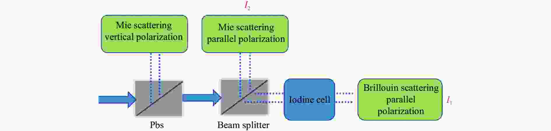
图 2 高光谱滤波模式
Figure 2. Hyperspectral mode of filtering
平行偏振通道散射光经过分束器,一部分通过碘池提取布里渊后向散射信号(以下简称布里渊通道),透过碘池的光强记为I1,如公式(3)所示;不通过碘池的通道可看作是颗粒物散射+瑞利散射+布里渊散射的总和(以下简称总和通道),其光强记为I2,如公式(4)所示:
$$ {{I}}_{1}=\int R\left(v\right) \cdot f\left(v\right){\rm{d}}v$$ (3) $$ {{I}}_{2}=\int R\left(v\right){\rm{d}}v $$ (4) 式中:
${R}\left({v}\right)$ 为回波信号光谱函数;${f}\left({v}\right)$ 为对应的碘分子吸收曲线函数。所示两个通道的信号强度之差${{I}}_{{{2}}}-{{I}}_{{{1}}}$ 为颗粒物后向散射+瑞利散射的结果。但是在大洋I类水体,相对于颗粒物散射,瑞利散射的结果通常要弱得多[14],所以可认为这个差值主要来源于平行通道POC散射的贡献。探测系统仿真用到的参数列表如表1所示。表 1 系统参数
Table 1. Parameters of lidar
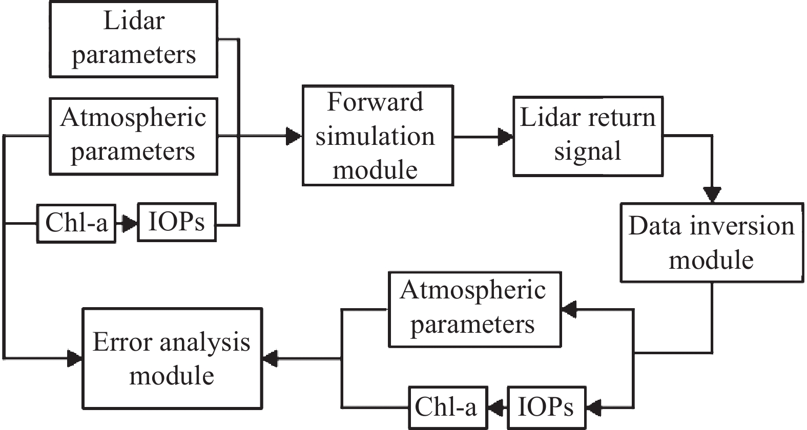
Parameter Value Wavelength $ \lambda $ 532.2 Lidar altitude ${ {H} }$ 2 000 Pulse energy $ E $ 1 Pulse repetition frequency/kHz 5 Pulse width $ \mathrm{\Delta }t $ 10 Receiver effective area A/m2 0.031 4 Refraction index $ n $ 1.35 Transmittance of the receiver optics ${T}_{{\rm{0}}}$ 0.5 Transmittance through the sea surface $ {T}_{s} $ 0.95 Quantum efficiency of PMT 0.1 Dynamic range of PMT/dB 50 Overlap factor $ O $ 1 Splitting ratio 1∶4 据雷达方程(公式(1))可知,海洋剖面回波信号强度与水体散射密切相关。使用中国海洋大学唐军武教授、刘秉义教授团队提供的星载海洋激光雷达仿真系统,可获得部分海域叶绿素剖面浓度信息,进而计算不同海域的水体参数剖面。仿真模拟系统的流程图如图3所示[13]。
通过扫描仿真海域的经纬度,在软件中获得叶绿素剖面浓度参数,进而用激光雷达方程计算回波光子剖面数据,最后根据信噪比和探测器单光子模式下的动态范围估算最大穿透深度。
假设激光雷达信号的信噪比为SNR,意味着激光雷达测量相对误差为
$1/{SNR}$ 。为使POC浓度数据反演百分比误差控制在30%以内,即需满足:$$ \sqrt{{{\sigma }_{{\rm{chl-a}}}}^{2}+{{\sigma }_{{\rm{bbp}}}}^{2}+{{\sigma }_{{\rm{POC}}}}^{2}+{\left(\frac{1}{SNR}\right)}^{2}}\leqslant 30{\text{%}} $$ (5) 根据公式(5)可知,信噪比需满足
$ SNR\geqslant 4.5 $ 。方便起见,取单次探测系统信噪比为5(即单次探测回波$ SNR=\sqrt{{N}_{phoele}}=25 $ 个光电子),根据激光雷达方程计算可得到回波光电子数随深度的变化图。假定光电探测器动态范围为50 dB,依据该动态范围,判断能够穿透的最大深度${H}_{{\rm{max}}}$ 。${H}_{{\rm{max}}}$ 的定义如下:$$ 10\cdot\mathrm{log}\left(\frac{{N}_{{H}_{{\rm{max}}}}}{{N}_{{H}_{0}}}\right)=50\;{\rm{dB}} $$ (6) 式中:
$N_{H_0}$ 为海平面处的回波光电子数;$N_{H_{{\rm{max}}}}$ 为最大穿透深度处的回波光电子数。由此估算探测系统在不同海域的最大探测深度如图4所示。图4中,横纵坐标为经纬度,其中东经、北纬为正;西经、南纬为负。由图4(a)、(b)可知,探测系统在印度洋海域最大探测深度为80 m,在南太平洋海域可探测90 m。2020年,Liu Qun等人[12]计算的星载激光雷达最大可探测海洋深度结果如图4(c)所示。由于仿真模拟系统海洋水体数据有限,其中红色框内为文中所估算的海域。与Liu Qun等人估算的结果比较,相同海域最大可探测深度与分布基本一致,具体结果存在一定误差的原因可能是搭载平台以及系统参数设置的不同。

图 4 (a)部分印度洋海域最大探测深度;(b)部分南太平洋海域最大探测深度;(c) Liu Qun等人估算星载海洋激光雷达最大探测海洋深度[12]
Figure 4. (a) Maximum sounding depth in some waters of the Indian Ocean; (b) Maximum sounding depth in some waters of the South Pacific Ocean; (c) Maximum ocean depth estimation using space-based ocean lidar, Liu Qun et al[12]
在实际激光雷达系统中,可参考以上信息选择合适的海域进行探测。
-
激光雷达的波长是一个重要的参数,它直接影响回波信号的处理以及剖面信息的反演。考虑到工程难度以及保证激光雷达使用的稳定性,必须在系统设计初期确定最佳的工作波长。碘分子气体吸收池在532 nm附近有多条吸收线,其中 1104~1112 线对应的基频对于 Nd:YAG 激光器都相对容易获得[16],因此成为基于碘分子的高光谱分辨率激光雷达最佳工作波长的待选范围。
激光雷达系统不同的载荷平台导致了回波信号光谱存在一定差异,船载平台只需考虑激光脉冲在海水中的传输特性即可,机载平台则需同时考虑激光脉冲在空气及海水中的传播特性。相应的选择碘分子吸收曲线及激光器的中心波长会有所差别。下面将通过仿真分别讨论两种平台下激光雷达系统最佳工作波长的选择。
-

由图5可知,回波光谱中包含发生频移的分子布里渊散射信号和不发生频移的颗粒物散射信号。因此,要获取海洋颗粒物的剖面浓度信息,需要利用碘分子气体吸收池滤波,原理如图1所示。
为实现有效滤波,船载系统波长的选择原则如下:
(1)在激光器中心波长处的碘分子池吸收率尽可能大,以尽可能将POC米散射信号吸收干净;
(2)布里渊频移会随温度而改变,海水温度范围约为4~30 ℃,对应的布里渊频移约为7.4~7.8 GHz,在该频移范围内,要求碘分子吸收曲线对布里渊信号的吸收率尽可能低、尽可能保证分子散射信号通过;
(3)实际应用中,激光器中心波长随着使用时长以及其他原因会存在一定的漂移,在激光器的中心波长尽可能大的漂移范围内,I2–I1的变化应尽可能小,以保证使用的稳定性。
为便于模拟,预设了一些初始参数,分别是盐度35‰、米散射峰半高全宽60 MHz、布里渊频移7.4~7.8 GHz。碘分子吸收曲线受到温度、压强、以及碘池长度的影响。这里将碘池参数设置为温度343 K、长度10.16 cm、压强1 torr (1 torr=133.322 Pa)。基于以上选择原则及碘池参数进行仿真分析。
当激光器中心波长为532.2451 nm、频率抖动范围±90 MHz 时,I2–I1随温度的变化曲线如图6所示。从图中可以看出,I2–I1的归一化强度随着温度的升高先下降后上升,当激光器的中心频率发生一定漂移时,I2–I1的归一化强度也存在一定的变化。相校中心波长532.2451 nm,当归一化强度发生5‰变化,对应的中心频率抖动范围为±90 MHz。同理,其他碘池吸收线的特性总结如表2所示。
表 2 船载探测系统不同工作波长的特性
Table 2. Characteristics of the different operating wavelengths of the shipboard detection system
Wavelength/nm Line Center frequency jitter range at 5‰
error of normalized intensity/MHz532.1985 - ±60 532.2423 1111 ±30 532.2451 1110 ±90 532.2897 1105 ±30 532.2928 1104 ±60 
图 6 中心频率抖动下,归一化强度随温度的变化
Figure 6. Variation of normalized intensity with temperature under central frequency dithering
从允许中心波长抖动范围的角度看,1110吸收线对应的532.2451 nm在船载系统最具优势;1104吸收线对应的中心波长532.2928 nm以及532.1985 nm次之。
-
若激光雷达系统使用机载平台,激光传输路径需同时考虑大气和海洋的影响。海洋通道可参照2.2.1节。
激光在大气中的散射光谱主要是由散射粒子的多普勒展宽引起的。大气分子的热运动高达几百米/s,导致分子瑞利散射光谱宽度达到 GHz 量级[18]。激光雷达系统接收端所接收到的回波信号频谱如图7所示[18]。

图 7 HSRL返回光谱的示意图
Figure 7. Schematic diagram for an HSRL return spectra
回波信号通过碘池后,大部分米散射信号将被滤除。分子散射信号的吸收率可以表示为:
$$ {{T}}_{{m}}=1-\frac{\displaystyle\int {R}_{m}\left({v}\right) \cdot f\left(v\right){\rm{d}}v}{\displaystyle\int {R}_{m}\left(v\right){\rm{d}}v} $$ (7) 颗粒物散射信号的吸收率可以表示为:
$$ {{T}}_{{a}}=1-\frac{\displaystyle\int {R}_{a}\left({v}\right) \cdot f\left(v\right){\rm{d}}v}{\displaystyle\int {R}_{a}\left(v\right){\rm{d}}v} $$ (8) 由于激光在大气中传输的特殊性,在机载系统中碘分子吸收曲线中心波长的选择要考虑到消光比,一般需要达到25~30 dB。消光比的计算如下:
$$ {E}{X}=10 \cdot \mathrm{log}\left(\frac{\displaystyle\int {R}_{a}\left(v\right){\rm{d}}v}{\displaystyle\int {R}_{a}\left({v}\right) \cdot f\left(v\right){\rm{d}}v}\right) $$ (9) 式中:
$ {R}_{m}\left(v\right) $ 为分子散射信号光谱函数;$ {R}_{a}\left(v\right) $ 为颗粒物散射信号光谱函数;$ f\left(v\right) $ 为碘分子吸收曲线函数。理想的碘分子滤波器应使颗粒物散射吸收率尽可能大,中心波长抖动带来的颗粒物吸收率的变化尽可能小,同时分子散射吸收率尽可能小。各吸收线仿真结果如表3所示。表 3 机载探测系统不同工作波长的特性
Table 3. Characteristics of the different operating wavelengths of the airborne detection system
Wavelength/
nmExtinction ratio/
dBFWHM/
GHzLine $ {T}_{m};{T}_{a} $ Normalization intensity
change (4-32 ℃)$ {T}_{m};{T}_{a} $ change
(±60 MHz)Normalization intensity
change (±60 MHz)532.1985 28.8 1.42 - 64.4%; 99.5% 3‰ 17.8‰; 2.4‰ 3‰ 532.2451 30.2 1.28 1110 58.5%; 99.8% 2‰ 2.9‰; 0.8‰ 5‰ 532.2897 25.9 1.28 1105 56.7%; 99.5% 2‰ 0.7‰; 2.1‰ 4‰ 532.2928 30.9 1.40 1104 60.8%; 99.8% 5‰ 1.3‰; 0.3‰ 5‰ 表3中列出了每个待选中心波长处的消光比、分子、颗粒物散射吸收率、4~32 ℃时海洋通道I2–I1的归一化强度变化范围,以及中心频率抖动时的表现。表3中四个中心波长均满足大气通道消光比要求,考虑大气通道时中心频率稳定性的要求,可以看到,532.1985 nm在频率发生抖动时,分子、颗粒物吸收率均有较大变化,故不作备选;结合表2中的结果,532.2897 nm 对应的1105吸收线频率稳定性不够理想,故不作备选。综上,1104吸收线以及1110吸收线不论是在海洋通道还是大气通道均有较优秀的性能表现。
-
目前海洋POC探测的需求迫切,海洋激光雷达系统因其优势可实现干净大洋水体的探测。文中从激光雷达方程入手,估算了大洋水体理论条件下最大可探测深度。基于碘池的高光谱分辨率探测技术,结果表明探测深度受海洋水体影响较大,干净大洋水体50 dB动态范围可达到80 m。此外,基于工作中心波长满足设计要求且具有高稳定性原则,碘池在532 nm附近的1104吸收线对应532.2928 nm,1110吸收线对应532.2451 nm,在海洋通道和大气通道符合文中设计要求,均可作为船载以及机载激光雷达系统的最佳工作中心波长。该工作主要对海洋有机碳剖面探测激光雷达系统进行了性能仿真分析,为后续碳剖面激光雷达探测系统的实际应用提供了设计参考。
Simulation of high spectral resolution oceanic particulate carbon profile detection system
-
摘要: 海洋是全球碳循环过程中的重要环节,从浮游植物光合作用开始,碳在海洋中沿食物链传递,以颗粒有机碳(POC)形式存在。对海洋中颗粒有机碳含量的探测,将对海洋碳汇能力的评估起到重要作用。在干净大洋水体中,激光雷达可根据浮游植物引起的光学性质变化实现剖面信息的探测,因此对基于高光谱分辨率技术的海洋颗粒有机碳浓度剖面探测系统性能进行了仿真分析。利用激光雷达方程对探测系统在大洋水体的最大探测深度进行了仿真;利用碘分子吸收池作滤波器,并结合大洋水体的透射窗口和激光器的工程设计,分析了不同载荷平台下探测系统的最佳工作波长。仿真结果表明,在满足单次探测系统信噪比为5的探测要求时,大洋水体50 dB动态范围下的探测深度平均在80 m;船载、机载平台探测系统最佳工作波长为532.245 1 nm和532.292 8 nm。Abstract:
Objective The ocean is an important link in the global carbon cycle, carbon is transferred along the ocean's food chain starting with phytoplankton photosynthesis and exists as particulate organic carbon (POC). The measurement of the ocean's ability to store carbon will be greatly influenced by the discovery of its particulate organic carbon content. The realization of ocean particulate matter profiling can clarify the key processes of its formation, evolution and transport, which is of great significance to regional and global ecological research and climate problem solution. It will help human beings to better understand the ocean and explore its deep resources. Half of the current contribution to ocean observation data comes from satellite remote sensing, a technique that allows simultaneous observation of large areas, but lacks access to ocean profile information. The performance of the oceanic particulate organic carbon concentration profile detection system based on high spectral resolution technology is simulated and analyzed because lidar can detect profile information based on the change in optical properties caused by phytoplankton in clear ocean waters. Methods High Spectral Resolution Lidar (HSRL) is a type of lidar that uses narrowband filters (or filters) to achieve spectral separation by taking advantage of the difference in the magnitude of the spectral width of particle scattering and molecular scattering in the backscattering spectrum of the echo signal (Fig.1). HSRL technology is the current preferred solution for the development of particle detection lidar. The simulation software (Fig.2) is used to obtain the ocean water parameters combined with the preset lidar system parameters (Tab.1), and then the lidar equation is used to simulate the return profile photoelectron number. Utilizing an iodine molecular absorption cell as a filter, the transmission window of the oceanic water column, and the laser's engineering design are combined to analyze the detection system's optimal operating wavelength under various loading platforms. Results and Discussions When the detection requirement of a single detection system with a signal-to-noise ratio of 5 is met, simulation results reveal that the detection depth in the 50 dB dynamic range of the oceanic water column averages at 80 m (Fig.4). Depending on the return spectrum (Fig.5, Fig.7) and filtering capabilities of the filter, the best center wavelength for lidar operation in various usage scenarios can be chosen. The absorption line of the iodine molecule absorption cell near 532 nm can be used as the working wavelength to be selected. The optimal operating center wavelength of the shipboard platform needs to consider the transmission characteristics of the laser in seawater (Tab.2). The optimal operating center wavelength of the airborne platform needs to take into account the atmospheric transmission characteristics of the laser (Tab.3). According to the filter's ability to absorb the meter scattered signal in the echo spectrum, and the stability requirements, the most effective working wavelength for airborne detection systems and shipborne detection systems is 532.292 8 nm and 532.245 1 nm. Conclusions Because the development of a lidar system is a time-consuming and difficult project, it is essential to simulate and optimize the system parameters early on to ensure the viability and usability of the lidar system. The water body has an effect on the maximum detectable depth of lidar, according to simulation results. The actual ocean exploration can choose the appropriate sea area to obtain better results. The determination of the optimal operating wavelength for high spectral resolution lidar based on iodine molecular absorption cell can provide a reference for the subsequent construction of practical systems. -
Key words:
- lidar /
- ocean POC detection /
- iodine pool filter /
- performance simulation
-
图 1 碘分子吸收池高光谱分辨率探测原理
Figure 1. High spectral resolution detection principle for iodine molecular absorption cells
图 4 (a)部分印度洋海域最大探测深度;(b)部分南太平洋海域最大探测深度;(c) Liu Qun等人估算星载海洋激光雷达最大探测海洋深度[12]
Figure 4. (a) Maximum sounding depth in some waters of the Indian Ocean; (b) Maximum sounding depth in some waters of the South Pacific Ocean; (c) Maximum ocean depth estimation using space-based ocean lidar, Liu Qun et al[12]
图 6 中心频率抖动下,归一化强度随温度的变化
Figure 6. Variation of normalized intensity with temperature under central frequency dithering
表 1 系统参数
Table 1. Parameters of lidar
Parameter Value Wavelength $ \lambda $/nm 532.2 Lidar altitude ${ {H} }$/m 2 000 Pulse energy $ E $/μJ 1 Pulse repetition frequency/kHz 5 Pulse width $ \mathrm{\Delta }t $/ns 10 Receiver effective area A/m2 0.031 4 Refraction index $ n $ 1.35 Transmittance of the receiver optics ${T}_{{\rm{0}}}$ 0.5 Transmittance through the sea surface $ {T}_{s} $ 0.95 Quantum efficiency of PMT 0.1 Dynamic range of PMT/dB 50 Overlap factor $ O $ 1 Splitting ratio 1∶4  下载: 导出CSV
表 2 船载探测系统不同工作波长的特性
Table 2. Characteristics of the different operating wavelengths of the shipboard detection system
Wavelength/nm Line Center frequency jitter range at 5‰
error of normalized intensity/MHz532.1985 - ±60 532.2423 1111 ±30 532.2451 1110 ±90 532.2897 1105 ±30 532.2928 1104 ±60
下载: 导出CSV
表 3 机载探测系统不同工作波长的特性
Table 3. Characteristics of the different operating wavelengths of the airborne detection system
Wavelength/
nmExtinction ratio/
dBFWHM/
GHzLine $ {T}_{m};{T}_{a} $ Normalization intensity
change (4-32 ℃)$ {T}_{m};{T}_{a} $ change
(±60 MHz)Normalization intensity
change (±60 MHz)532.1985 28.8 1.42 - 64.4%; 99.5% 3‰ 17.8‰; 2.4‰ 3‰ 532.2451 30.2 1.28 1110 58.5%; 99.8% 2‰ 2.9‰; 0.8‰ 5‰ 532.2897 25.9 1.28 1105 56.7%; 99.5% 2‰ 0.7‰; 2.1‰ 4‰ 532.2928 30.9 1.40 1104 60.8%; 99.8% 5‰ 1.3‰; 0.3‰ 5‰
下载: 导出CSV
-
[1] 柴麒敏, 郭虹宇, 刘昌义, 等. 全球气候变化与中国行动方案——“十四五”规划期间中国气候治理(笔谈)[J]. 阅江学刊, 2020, 12(6): 36-58. doi: 10.13878/j.cnki.yjxk.20210107.001 [2] Zhou Chenhao, Mao Qinyu, Xu Xiao, et al. Preliminary analysis of C sequestration potential of blue carbon ecosystems on Chinese coastal zone [J]. Scientia Sinica Vitae, 2016, 46(4): 475-486. (in Chinese) doi: 10.1360/N052016-00105 [3] Jiang Xingwei, He Xianqiang, Lin Mingsen, et al. Progress on ocean satellite remote sensing application in China [J]. Haiyang Xuebao, 2019, 41(10): 113-124. (in Chinese) doi: 10.3969/j.issn.0253−4193.2019.10.007 [4] Tang Junwu, Chen Ge, Chen Weibiao, et al. Three dimensional remote sensing for oceanography and the Guanlan ocean profiling Lidar [J]. National Remote Sensing Bulletin, 2021, 25(1): 460-500. (in Chinese) [5] Zhu Shouzheng, Bu Lingbing, Liu Jiqiao, et al. Study on airborne high spectral resolution lidar detection optical properties and pollution of atmospheric aerosol [J]. Chinese Journal of Lasers, 2021, 48(17): 1710003. (in Chinese) [6] Schulien J A, Behrenfeld M J, Hair J W, et al. Vertically-resolved phytoplankton carbon and net primary production from a high spectral resolution lidar [J]. Optics Express, 2017, 25(12): 13577-13587. doi: 10.1364/OE.25.013577 [7] Schulien J A, Penna A D, Gaube P, et al. Shifts in phytoplankton community structure across an anticyclonic eddy revealed from high spectral resolution lidar scattering measurements [J]. Frontiers in Marine Science, 2020, 7: 493. [8] Liu Zhipeng, Liu Dong, Xu Peituo, et al. Retrieval of seawater optical properties with an oceanic lidar [J]. Journal of Remote Sensing, 2019, 23(5): 944-951. (in Chinese) [9] Zhou Yudi, Liu Dong, Xu Peituo, et al. Detection atmospheric-water optical property profiles with a polarized lidar [J]. Journal of Remote Sensing, 2019, 23(1): 108-115. (in Chinese) [10] He Yan, Hu Shanjiang, Chen WeiBiao, et al. Research progress of domestic Airborne Dual-Frequency Lidar detection technology [J]. Laser and Optoelectronics Progress, 2018, 55(8): 082801. (in Chinese) [11] Hu Shanjian, He Yan, Chen Weibiao, et al. Design of airbone dual-frequency laser radar system [J]. Infrared and Laser Engineering, 2018, 47(9): 0930001. (in Chinese) doi: 10.3788/IRLA201847.0930001 [12] Liu Q, Liu D, Zhu X, et al. Optimum wavelength of spaceborne oceanic lidar in penetration depth [J]. Journal of Quantitative Spectroscopy and Radiative Transfer, 2020, 256: 107310. doi: 10.1016/j.jqsrt.2020.107310 [13] Zhu Peizhi, Liu Bingyi, Kong Xiaojuan, et al. Estimation of chlorophyll profile detection capability of spaceborne oceanographic lidar [J]. Infrared and Laser Engineering, 2021, 50(2): 20200164. (in Chinese) doi: 10.3788/IRLA20200164 [14] Jerlov N G. Marine Optics [M]. Amsterdam: Elsevier, 1976. [15] Tang Junwu, Zhu Peizhi, Liu Bingyi, et al. Polarized light scattering of particulate matter in detection of oceanographic profiling lidar [J]. Acta Optica Sinica, 2022, 42(12): 1200001. (in Chinese) [16] She C Y. Spectral structure of laser light scattering revisited: bandwidths of nonresonant scattering lidars [J]. Applied Optics, 2001, 40(27): 4875-4884. doi: 10.1364/AO.40.004875 [17] Xu Jiaqi, Wang Yuanqing, Xu Yangrui, et al. Research progress of ocean environment laser remote sensing based on Brillion scattering [J]. Infrared and Laser Engineering, 2021, 50(6): 20211036. (in Chinese) doi: 10.3788/IRLA20211036 [18] Zhang Yupeng, Liu Dong, Shen Xue, et al. Design of iodine absorption cell for high-spectral-resolution lidar [J]. Optics Express, 2017, 25(14): 15913-15926. -

 点击查看大图
计量
- 文章访问数: 65
- HTML全文浏览量: 16
- PDF下载量: 26
- 被引次数: 0


