


-
光学频率梳(Optical Frequency Comb, OFC)广泛应用于光谱学、光通信、测距等领域[1-4]。使用光学谐振器、锁模激光器和电光调制器(Electro-Optic Modulator, EOM)是产生光学频率梳的主要方法[5]。
基于电光调制产生光学频率梳的方法可采用相位调制器(Phase Modulator, PM)、强度调制器(Intensity Modulator, IM)和双平行马赫-曾德尔调制器(Dual Parallel Mach-Zehnder Modulator, DPMZM)。其基本原理是通过正弦波驱动铌酸锂相位调制器,产生大量边带,再通过不同相位调制的光信号之间的叠加与级联,得到谱线范围宽、平坦度好的光学频率梳[6-9]。在这一过程中,需要调整电光调制器驱动信号的相位。参考文献[10]研究了使用单个相位调制器产生平坦光学频率梳的方法。该方法让基频和三次谐波调制光载波相位,通过调整两个驱动信号的调制指数和相位,得到平坦度为0.8 dB的9根谱线光学频率梳。但是在该方法下相位变化限于固定的90°,没有进一步通过优化驱动信号相位改善光学频率梳的平坦度和光谱宽度性能。参考文献[11]提出了使用双平行马赫-曾德尔调制器产生平坦光学频率梳的方法。该方法使用单个微波信号驱动双平行马赫-曾德尔调制器的一个子马赫-曾德尔调制器,通过调整双平行马赫-曾德尔调制器上三个偏置电压实现平坦度不超过1 dB的7根谱线光学频率梳。参考文献[12]使用一个微波信号驱动双偏振正交相移键控调制器,产生了平坦度为1.12 dB、9根谱线的光学频率梳。同一课题组同年提出使用双驱动马赫-曾德尔调制器产生平坦光学频率梳的方法,该方法通过单一微波信号驱动调制器产生了平坦度为0.7 dB的20根谱线光学频率梳[13]。但是以上这些方法都没有通过优化驱动信号相位得到性能更好的光学频率梳。
参考文献[14]提出了使用一个强度调制器和两个相位调制器级联的方式来产生光学频率梳的方法,其驱动信号是单个微波信号。该方法通过调整驱动相位调制器的微波信号相位和强度调制器的偏置电压,产生了平坦度不超过1.5 dB的29根谱线光学频率梳,但是该方法没有进一步优化平坦度性能。参考文献[15]使用叠加的谐波驱动级联的相位调制器的方法产生平坦的光学频率梳。该方法优化了微波驱动信号的相位,产生了平坦度为0.65 dB的15根谱线光学频率梳,但是该方法没有研究固定某一微波驱动信号相位对于生成的平坦光学频率梳性能的影响。
针对上述问题,文中提出了使用叠加谐波驱动级联相位调制器和强度调制器产生平坦光学频率梳的方法。该方法以最小化平坦光学频率梳功率方差为目标,通过差分进化算法,得到优化后的驱动信号调制指数和相位以及强度调制器偏置电压带来的偏置相位,进而得到文中方法下微波驱动信号的叠加方案及其产生的平坦光学频率梳性能。当固定某个微波驱动信号的相位时,以上优化方法依然可以生成平坦的光学频率梳,这提高了该方法的鲁棒性。相关理论分析得到了实验验证。当使用叠加的基频和三次谐波驱动相位调制器、使用四次谐波驱动强度调制器时,可分别通过仿真和实验得到平坦度为0.27 dB和0.83 dB的13根谱线光学频率梳。实验图与仿真图趋势一致,证实了所提方法的可行性。
-
文中通过叠加微波信号驱动级联的相位调制器和强度调制器,根据优化设计得到的微波信号调制指数和相位以及强度调制器的偏置相位等参数,生成平坦光学频率梳,其原理图如图1所示。激光器(Laser Diode, LD)输出连续光的电场用
$ {E}_{\mathrm{L}\mathrm{D}}\left(t\right) $ 描述: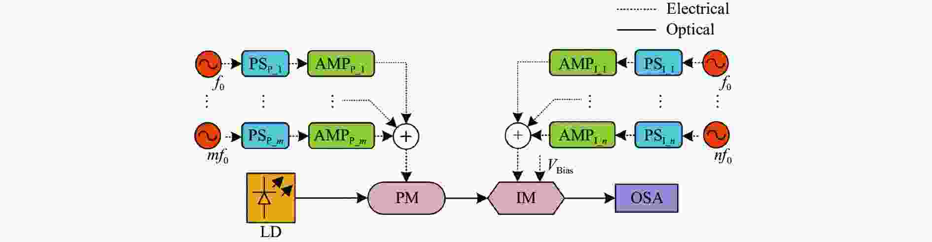
图 1 使用级联相位调制器和强度调制器产生平坦光学频率梳的方法
Figure 1. Schematic to generate flat OFC by using cascaded PM and IM
$$ {E}_{\mathrm{L}\mathrm{D}}\left(t\right)={E}_{\mathrm{c}}{{\rm{e}}}^{j2\mathrm{\pi }{f}_{\mathrm{c}}t} $$ (1) 式中:
$ {E}_{\mathrm{c}} $ 和$ {f}_{\mathrm{c}} $ 分别为连续光的电场幅度和工作频率。当连续光通过相位调制器时,其输出光场为:$$ {E}_{\mathrm{P}\mathrm{M}}\left(t\right)={E}_{\mathrm{L}\mathrm{D}}\left(t\right){{\rm{e}}}^{j{s}_{\mathrm{P}\mathrm{M}}\left(t\right)} $$ (2) 式中:
$ {s}_{\mathrm{P}\mathrm{M}}\left(t\right) $ 为相位调制器的驱动信号。如图1所示,该驱动信号可表示为:$$ {s}_{\mathrm{P}\mathrm{M}}\left(t\right)=\sum \nolimits_{i}{\,\beta }_{\mathrm{P}\mathrm{M},i}\mathrm{cos}\left(2\pi i{f}_{0}t+{\varphi }_{\mathrm{P}\mathrm{M},i}\right) $$ (3) 式中:
$ {f}_{0} $ 为谐波信号的基频;$ i $ 为$ \left\{1,2,\cdots ,m\right\} $ 内的某几个整数;$ {\varphi }_{\mathrm{P}\mathrm{M},i} $ 和$ {\,\beta }_{\mathrm{P}\mathrm{M},i} $ 分别为第$ i $ 次谐波的相位和调制指数;$ {\,\beta }_{\mathrm{P}\mathrm{M},i}=\pi \dfrac{{V}_{\mathrm{P}\mathrm{M},i}}{{V}_{\pi }} $ 为相位调制器的调制指数,$ {V}_{\mathrm{P}\mathrm{M},i} $ 为第$ i $ 次谐波的幅度,$ {V}_{\pi } $ 是相位调制器的半波电压[16-17]。根据Jacobi-Anger展开式[18-19],可知:$$ \begin{split} {{\rm{e}}}^{j{s}_{\mathrm{P}\mathrm{M}}\left(t\right)}=&{{\rm{e}}}^{j\sum _{i}{\,\beta }_{\mathrm{P}\mathrm{M},i}\mathrm{cos}\left(2\pi i{f}_{0}t+{\varphi }_{\mathrm{P}\mathrm{M},i}\right)} =\\& \prod _{i}\sum _{{k}_{i}=-\infty }^{\infty }{j}^{{k}_{i}}{J}_{{k}_{i}}\left({\,\beta }_{\mathrm{P}\mathrm{M},i}\right){\rm e}^{j{k}_{i}\left(2\pi i{f}_{0}t+{\varphi }_{\mathrm{P}\mathrm{M},i}\right)} \end{split} $$ (4) 则公式(2)描述的相位调制后的光场频谱可表示为:
$$ \begin{split} {\tilde{E}}_{\mathrm{P}\mathrm{M}}\left(f\right)=&{E}_{{{{c}}}}\left[\prod _{i}\sum _{{k}_{i}=-\infty }^{\infty }{j}^{{k}_{i}}{J}_{{k}_{i}}\left({\,\beta }_{\mathrm{P}\mathrm{M},i}\right){\rm e}^{j{k}_{i}{\varphi }_{\mathrm{P}\mathrm{M},i}}\right] \cdot\\& \left[{\otimes }_{i}\delta \left(f-{ik}_{i}{f}_{0}\right)\right]\otimes \delta \left(f-{f}_{{{c}}}\right) \end{split} $$ (5) 式中:
$ \otimes $ 代表卷积;$ {\otimes }_{i} $ 代表连续卷积;$ \tilde{E}\left(f\right) $ 表示傅里叶变换。当相位调制器的输出光通过强度调制器时,其被分成两路通过马赫-曾德尔干涉仪(Mach-Zehnder Interferometerer MZI)的结构。强度调制器输出光的电场可以表示为:
$$ {E}_{\mathrm{P}\mathrm{M}-\mathrm{I}\mathrm{M}}\left(t\right) =\frac{1}{\sqrt{2}}{E}_{\mathrm{P}\mathrm{M}}\left(t\right)\left[{{\rm{e}}}^{j{s}_{\mathrm{I}\mathrm{M}}\left(t\right)+j{\varphi }_{\mathrm{B}\mathrm{i}\mathrm{a}\mathrm{s}}}+{{\rm{e}}}^{-j{s}_{\mathrm{I}\mathrm{M}}\left(t\right)}\right] $$ (6) 式中:
$ {\varphi }_{\mathrm{B}\mathrm{i}\mathrm{a}\mathrm{s}} $ 为强度调制器偏置电压$ {V}_{\mathrm{B}\mathrm{i}\mathrm{a}\mathrm{s}} $ 带来的偏置相位。如图1所示,公式(6)中强度调制器的驱动信号$ {s}_{\mathrm{I}\mathrm{M}}\left(t\right) $ 可表示为:$$ {s}_{\mathrm{I}\mathrm{M}}\left(t\right)=\sum \nolimits_{\ell}{\,\beta }_{\mathrm{I}\mathrm{M},\ell}\mathrm{cos}\left(2\pi \ell{f}_{0}t+{\varphi }_{\mathrm{I}\mathrm{M},\ell}\right) $$ (7) 式中:
$ \ell $ 为$ \left\{1,2,\cdots ,n\right\} $ 内的某几个整数;$ {\,\beta }_{\mathrm{I}\mathrm{M},\ell} $ 为第$ \ell $ 次谐波对于该路相位调制过程的调制指数;$ {\varphi }_{\mathrm{I}\mathrm{M},\ell} $ 为第$ \ell $ 次谐波的相位。用$ {E}_{\mathrm{I}\mathrm{M}}\left(t\right) $ 表示公式(6)中的${{\rm{e}}}^{j{s}_{\mathrm{I}\mathrm{M}}\left(t\right)+j{\varphi }_{\mathrm{B}\mathrm{i}\mathrm{a}\mathrm{s}}}+ {{\rm{e}}}^{-j{s}_{\mathrm{I}\mathrm{M}}\left(t\right)}$ ,则根据Jacobi-Anger展开式可得:$$ {E}_{\mathrm{I}\mathrm{M}}\left(t\right)=\prod _{\ell}\sum _{{k}_{\ell}=-\mathcal{\infty }}^{\mathcal{\infty }}{j}^{{k}_{\ell}}{J}_{{k}_{\ell}}\left({\,\beta }_{\mathrm{I}\mathrm{M},\ell}\right){{\rm{e}}}^{j{k}_{\ell}{\varphi }_{\mathrm{I}\mathrm{M},\ell}}\left({{\rm{e}}}^{j{\varphi }_{\mathrm{B}\mathrm{i}\mathrm{a}\mathrm{s}}}+{{\rm{e}}}^{j{k}_{\ell}\pi }\right){{\rm{e}}}^{j2\pi \ell{k}_{\ell}{f}_{0}t} $$ (8) $ {E}_{\mathrm{I}\mathrm{M}}\left(t\right) $ 的频谱为:$$ \begin{split} {\tilde{E}}_{\mathrm{I}\mathrm{M}}\left(f\right)=&\left[\prod _{\ell }\sum _{{k}_{\ell }=-\mathcal{\infty }}^{\mathcal{\infty }}{j}^{{k}_{\ell }}{J}_{{k}_{\ell }}\left({\,\beta }_{\mathrm{I}\mathrm{M},\ell }\right){{\rm{e}}}^{j{k}_{\ell }{\varphi }_{\mathrm{I}\mathrm{M},\ell }}\left({{\rm{e}}}^{j{\varphi }_{\mathrm{B}\mathrm{i}\mathrm{a}\mathrm{s}}}+{{\rm{e}}}^{j{k}_{\ell }\pi }\right)\right]\cdot\\& \left[{\otimes }_{\ell }\delta \left(f-{\ell k}_{\ell }{f}_{0}\right)\right] \end{split} $$ (9) 由公式(6)可知
$ {E}_{\mathrm{P}\mathrm{M}-\mathrm{I}\mathrm{M}}\left(t\right)=\dfrac{1}{\sqrt{2}}{E}_{\mathrm{P}\mathrm{M}}\left(t\right){E}_{\mathrm{I}\mathrm{M}}\left(t\right) $ ,其频谱为:$$ \begin{split} & {\tilde{E}}_{\mathrm{P}\mathrm{M}-\mathrm{I}\mathrm{M}}\left(f\right)=\frac{1}{\sqrt{2}}{\tilde{E}}_{\mathrm{P}\mathrm{M}}\left(f\right)\otimes {\tilde{E}}_{\mathrm{I}\mathrm{M}}\left(f\right) =\\& \frac{1}{\sqrt{2}}{E}_{{c}}\left[\prod _{i}\sum _{{k}_{i}=-\infty }^{\infty }{j}^{{k}_{i}}{J}_{{k}_{i}}\left({\,\beta }_{\mathrm{P}\mathrm{M},i}\right){{\rm{e}}}^{j{k}_{i}{\varphi }_{\mathrm{P}\mathrm{M},i}}\right] \left[{\otimes }_{i}\delta \left(f-{ik}_{i}{f}_{0}\right)\right]\otimes\\& \delta \left(f-{f}_{c}\right)\otimes \left[\prod _{\ell}\sum _{{k}_{\ell}=-\mathcal{\infty }}^{\mathcal{\infty }}{j}^{{k}_{\ell}}{J}_{{k}_{\ell}}\left({\,\beta }_{\mathrm{I}\mathrm{M},\ell}\right){{\rm{e}}}^{j{k}_{\ell}{\varphi }_{\mathrm{I}\mathrm{M},\ell}}\left({{\rm{e}}}^{j{\varphi }_{\mathrm{B}\mathrm{i}\mathrm{a}\mathrm{s}}}+{{\rm{e}}}^{j{k}_{\ell}\pi }\right)\right]\cdot\\&\left[{\otimes }_{\ell}\delta \left(f-{\ell k}_{\ell}{f}_{0}\right)\right] \end{split} $$ (10) $ {\tilde{E}}_{\mathrm{P}\mathrm{M}-\mathrm{I}\mathrm{M}}\left(f\right) $ 的中心频率为$ {f}_{{c}} $ ,若要实现平坦的光学频率梳,则要对向量${\tilde{E}}_{\text{PM}-\text{IM}\text{,}\text{opt}}\left(f\right)=\left[{\tilde{E}}_{\mathrm{P}\mathrm{M}-\mathrm{I}\mathrm{M}}\left({f}_{{c}}-N{f}_{0}\right), \cdots , {\tilde{E}}_{\mathrm{P}\mathrm{M}-\mathrm{I}\mathrm{M}}\left({f}_{{c}}\right),\cdots ,{\tilde{E}}_{\mathrm{P}\mathrm{M}-\mathrm{I}\mathrm{M}}\left({f}_{{c}}+N{f}_{0}\right)\right]^{\mathrm{T}}$ 每根谱线的功率取对数后的方差进行最小化处理。该光学频率梳向量有$ 2 N+1 $ 个元素,考虑到器件的工作状态,上述调制指数参数不超过1.5,相位参数在0~$ 2\pi $ 之间变化。因此,相应的优化问题可写成公式(11)和公式(12):$$ P1:\mathrm{m}\mathrm{i}\mathrm{n}\mathrm{i}\mathrm{m}\mathrm{i}\mathrm{z}\mathrm{e}\;\;\mathrm{V}\mathrm{a}\mathrm{r}\left\{10{\mathrm{l}\mathrm{o}\mathrm{g}}_{10}{\left|{\tilde{E}}_{\text{PM}-\text{IM}\text{,}\text{opt}}\left(f\right)\right|}^{2}\right\} $$ (11) $$ \mathrm{s}\mathrm{u}\mathrm{b}\mathrm{j}\mathrm{e}\mathrm{c}\mathrm{t}\;\;\mathrm{t}\mathrm{o}\;\;0 < \,\beta \leqslant 1.5, 0 < \varphi \leqslant 2\pi $$ (12) 式中:
$ \mathrm{V}\mathrm{a}\mathrm{r} $ 表示取方差。 -
根据公式(11)描述的优化问题,使用差分进化算法得到微波驱动信号的调制指数
$ {\,\beta }_{\mathrm{P}\mathrm{M},i} $ 、$ {\,\beta }_{\mathrm{I}\mathrm{M},\ell } $ 和相应的相位$ {\varphi }_{\mathrm{P}\mathrm{M},i} $ 、$ {\varphi }_{\mathrm{I}\mathrm{M},\ell } $ 以及强度调制器的偏置相位$ {\varphi }_{\mathrm{B}\mathrm{i}\mathrm{a}\mathrm{s}} $ 等参数。在得到优化参数的过程中[20],如无其他说明,差分进化算法的参数如下。种群数量为500,最大进化代数为1000,变异因子(mutation constant)为0.5,交叉因子(crossover constant)为0.1。所得的产生平坦光学频率梳的叠加谐波组合及其优化参数见表1。表 1 产生平坦光学频率梳的叠加谐波组合
Table 1. Combinations of harmonics for the generation of flat OFC
Case Combined harmonics
that drive PMParameters of harmonics
that drive PMCombined harmonics
that drive IMParameters of harmonics
that drive IMNumber of
comb linesFlatness/dB (a) $ {f}_{0} $, $ 3{f}_{0} $ $ {\;\beta }_{\mathrm{P}\mathrm{M},1}= $1.50
$ {\;\beta }_{\mathrm{P}\mathrm{M},3}= $1.20
$ {\varphi }_{\mathrm{P}\mathrm{M},1}= $1.75
$ {\varphi }_{\mathrm{P}\mathrm{M},3}= $5.93$ 2{f}_{0} $ $ {\;\beta }_{\mathrm{I}\mathrm{M},2}= $0.45
$ {\varphi }_{\mathrm{I}\mathrm{M},2}= $3.05
$ {\varphi }_{\mathrm{B}\mathrm{i}\mathrm{a}\mathrm{s}}= $3.239 0.59 (b) $ {f}_{0} $, $ 3{f}_{0} $ $ {\;\beta }_{\mathrm{P}\mathrm{M},1}= $1.48
$ {\;\beta }_{\mathrm{P}\mathrm{M},3}= $1.12
$ {\varphi }_{\mathrm{P}\mathrm{M},1}= $3.01
$ {\varphi }_{\mathrm{P}\mathrm{M},3}= $3.85$ 4{f}_{0} $ $ {\;\beta }_{\mathrm{I}\mathrm{M},4}= $1.06
$ {\varphi }_{\mathrm{I}\mathrm{M},4}= $3.09
$ {\varphi }_{\mathrm{B}\mathrm{i}\mathrm{a}\mathrm{s}}= $2.9313 0.27 (c) $ {f}_{0} $, $ 3{f}_{0} $ $ {\;\beta }_{\mathrm{P}\mathrm{M},1}= $1.35
$ {\;\beta }_{\mathrm{P}\mathrm{M},3}= $0.92
$ {\varphi }_{\mathrm{P}\mathrm{M},1}= $3.32
$ {\varphi }_{\mathrm{P}\mathrm{M},3}= $5.20$ {f}_{0} $, $ 3{f}_{0} $, $ 5{f}_{0} $ $ {\;\beta }_{\mathrm{I}\mathrm{M},1}= $0.97
$ {\;\beta }_{\mathrm{I}\mathrm{M},3}= $0.63
$ {\;\beta }_{\mathrm{I}\mathrm{M},5}= $1.01
$ {\varphi }_{\mathrm{I}\mathrm{M},1}= $0.17
$ {\varphi }_{\mathrm{I}\mathrm{M},3}= $6.10
$ {\varphi }_{\mathrm{I}\mathrm{M},5}= $0.70
$ {\varphi }_{\mathrm{B}\mathrm{i}\mathrm{a}\mathrm{s}}= $3.1317 0.45 (d) $ {f}_{0} $, $ 3{f}_{0} $, $ 5{f}_{0} $ $ {\;\beta }_{\mathrm{P}\mathrm{M},1}= $1.36
$ {\;\beta }_{\mathrm{P}\mathrm{M},3}= $1.02
$ {\;\beta }_{\mathrm{P}\mathrm{M},5}= $1.06
$ {\varphi }_{\mathrm{P}\mathrm{M},1}= $4.34
$ {\varphi }_{\mathrm{P}\mathrm{M},3}= $5.18
$ {\varphi }_{\mathrm{P}\mathrm{M},5}= $2.44$ {f}_{0} $, $ 3{f}_{0} $, $ 5{f}_{0} $ $ {\;\beta }_{\mathrm{I}\mathrm{M},1}= $0.29
$ {\;\beta }_{\mathrm{I}\mathrm{M},3}= $1.04
$ {\;\beta }_{\mathrm{I}\mathrm{M},5}= $0.87
$ {\varphi }_{\mathrm{I}\mathrm{M},1}= $5.82
$ {\varphi }_{\mathrm{I}\mathrm{M},3}= $0.84
$ {\varphi }_{\mathrm{I}\mathrm{M},5}= $0.80
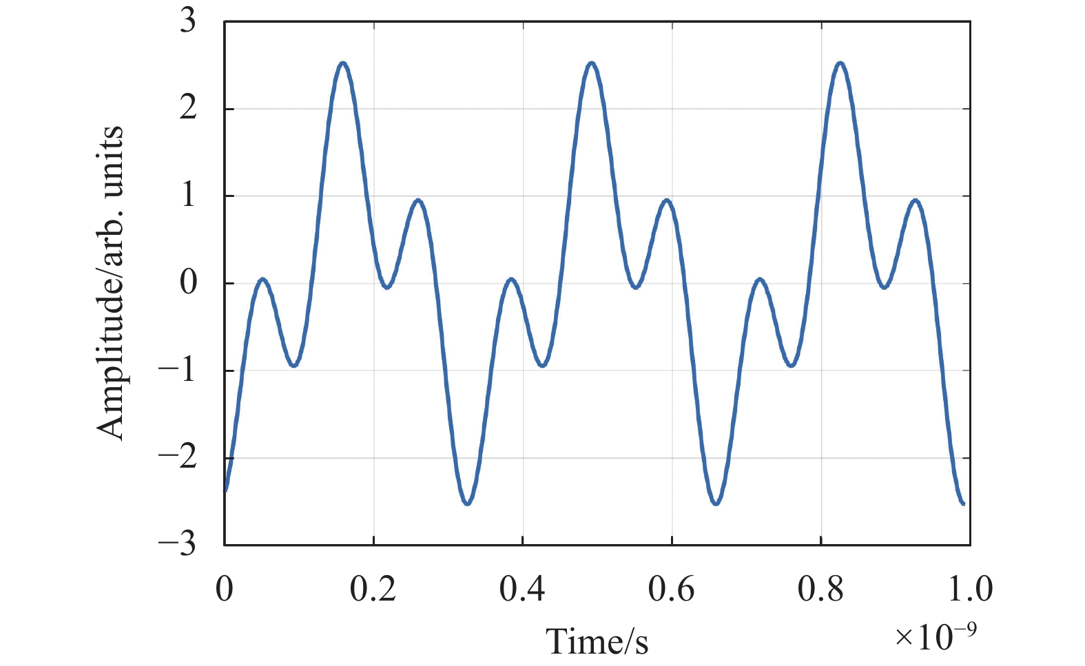
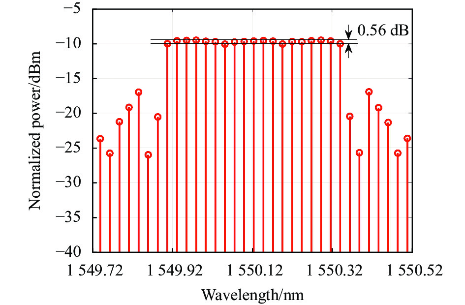
$ {\varphi }_{\mathrm{B}\mathrm{i}\mathrm{a}\mathrm{s}}= $0.0119 0.56 当使用叠加的基频和三次谐波驱动相位调制器、使用二次谐波驱动强度调制器时,可以得到平坦度为0.59 dB、9根谱线的光学频率梳。当相位调制器的驱动信号不变,强度调制器的驱动信号变为四次谐波时,可以得到平坦度为0.27 dB、13根谱线的光学频率梳。相应的驱动相位调制器的叠加谐波波形和平坦的光学频率梳仿真图分别如图2和图3所示。

图 2 驱动相位调制器的叠加的基频和三次谐波波形
Figure 2. Waveform of combined fundamental tone and third harmonic that drive the PM
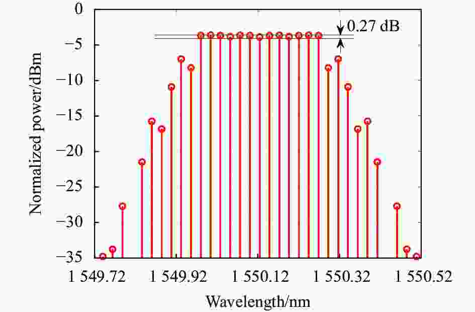
图 3 光学频率梳仿真图。基频、三次谐波驱动相位调制器,四次谐波驱动强度调制器
Figure 3. OFC in simulation, where the PM is driven by combined fundamental tone and third harmonic and the IM is driven by fourth harmonic
除了上述谐波组合外,其他谐波组合也可以在图1所示方法下实现平坦的光学频率梳。仿真结果显示,当叠加的基频和三次谐波驱动相位调制器,叠加的基频、三次谐波和五次谐波驱动强度调制器时,可以实现平坦度为0.45 dB的17根谱线光学频率梳;当叠加的基频、三次谐波、五次谐波驱动相位调制器和强度调制器时,可以实现平坦度为0.56 dB的19根谱线光学频率梳,如图4所示。

图 4 光学频率梳仿真图。基频、三次、五次谐波驱动相位调制器和强度调制器
Figure 4. OFC in simulation, where the combined fundamental tone, third and fifth harmonic drive both PM and IM
-
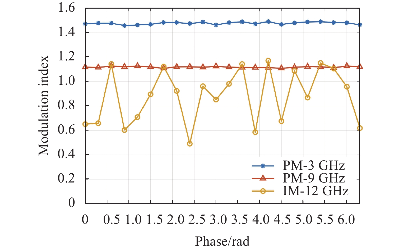
文中研究显示,对于公式(11)所描述的优化问题,当固定某一微波驱动信号的相位时,同样可以得到平坦的光学频率梳。以表1中的情况(b)为例进行讨论如下。
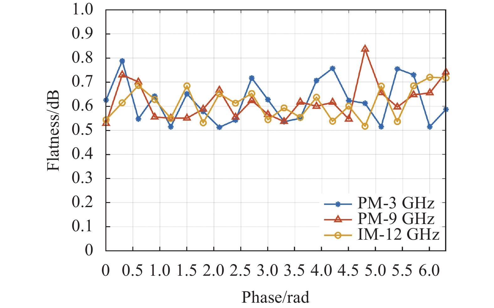
固定相位调制器驱动信号即3 GHz的基频信号、9 GHz的三次谐波和强度调制器驱动信号即12 GHz的四次谐波中任意一个微波信号的相位,使用差分进化算法求解公式(11)中的优化问题。之后在
$ \left[0,2\pi \right] $ 之间遍历$ {\varphi }_{\mathrm{P}\mathrm{M},1} $ 、$ {\varphi }_{\mathrm{P}\mathrm{M},3} $ 、$ {\varphi }_{\mathrm{I}\mathrm{M},4} $ ,得到平坦的光学频率梳和微波驱动信号相位之间的关系,如图5所示。当遍历$ {\varphi }_{\mathrm{P}\mathrm{M},1} $ 时,生成的光学频率梳的平坦度在0.22~0.46 dB之间变化;当遍历$ {\varphi }_{\mathrm{P}\mathrm{M},3} $ 时,生成的光学频率梳的平坦度在0.23~0.45 dB之间变化;当遍历$ {\varphi }_{\mathrm{I}\mathrm{M},4} $ 时,生成的光学频率梳平坦度在0.24~0.47 dB之间变化。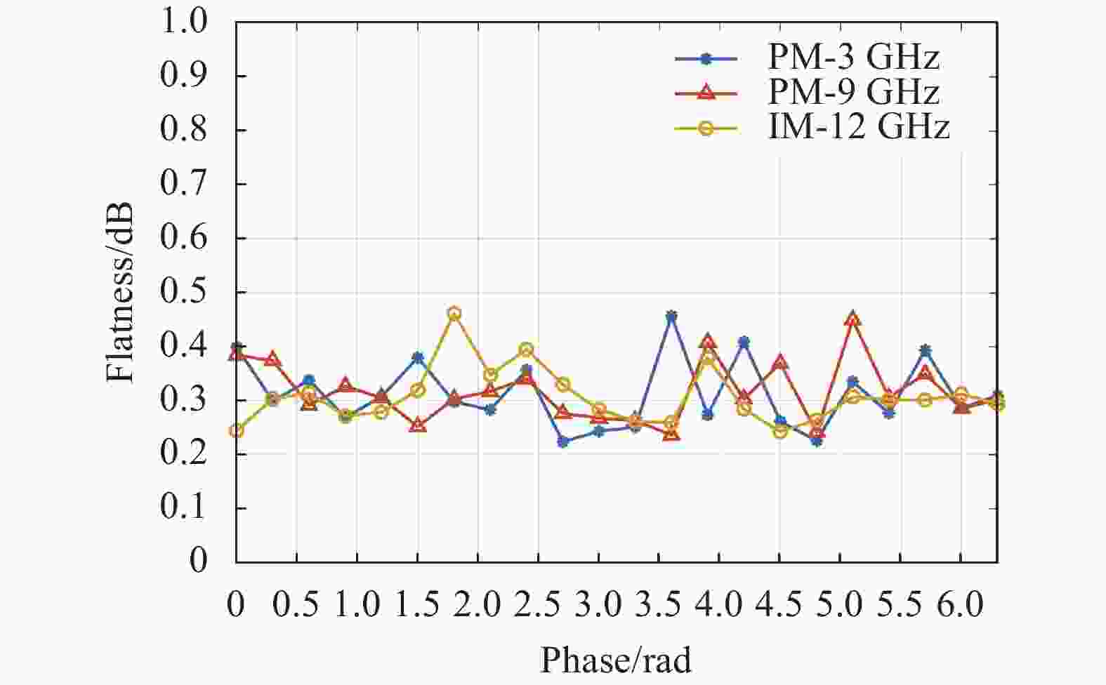
以下分析遍历
$ {\varphi }_{\mathrm{P}\mathrm{M},1} $ 、$ {\varphi }_{\mathrm{P}\mathrm{M},3} $ 、$ {\varphi }_{\mathrm{I}\mathrm{M},4} $ 时的各个微波驱动信号调制指数变化情况。如图6-8所示,当某个微波驱动信号相位固定时,相位调制器的两个驱动信号的调制指数基本不变,而强度调制器的驱动信号的调制指数则有较大的波动。当固定$ {\varphi }_{\mathrm{P}\mathrm{M},1} $ 时,相位调制器的3 GHz微波驱动信号的调制指数在1.46~1.50之间变化,相位调制器的9 GHz微波驱动信号的调制指数在1.10~1.13之间变化,强度调制器的12 GHz微波驱动信号的调制指数在0.52~1.20之间变化;当固定$ {\varphi }_{\mathrm{P}\mathrm{M},3} $ 时,3 GHz微波驱动信号的调制指数在1.45~1.50之间变化,9 GHz微波驱动信号的调制指数在1.10~1.13之间变化,12 GHz微波驱动信号的调制指数在0.49~1.18之间变化;当固定$ {\varphi }_{\mathrm{I}\mathrm{M},4} $ 时,3 GHz微波驱动信号的调制指数在1.45~1.50之间变化,9 GHz微波驱动信号的调制指数在1.10~1.14之间变化,12 GHz微波驱动信号的调制指数在0.57~1.20之间变化。

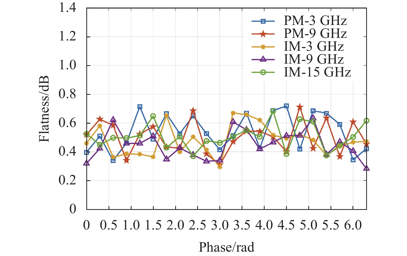
对于表1中的情况(c),在
$ \left[0,2\pi \right] $ 之间,分别遍历$ {\varphi }_{\mathrm{P}\mathrm{M},1} $ 、$ {\varphi }_{\mathrm{P}\mathrm{M},3} $ 、$ {\varphi }_{\mathrm{I}\mathrm{M},1} $ 、$ {\varphi }_{\mathrm{I}\mathrm{M},3} $ 、$ {\varphi }_{\mathrm{I}\mathrm{M},5} $ 得到光学频率梳的平坦度和固定的微波驱动信号相位的关系。如图9所示,光学频率梳平坦度的波动范围不超过0.41 dB,能够保证文中方法的鲁棒性。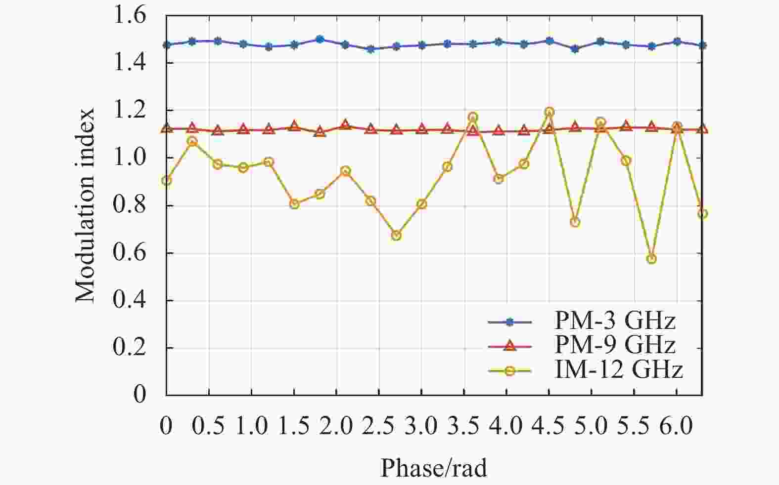

对于表1中的情况(a),在
$ \left[0,2\pi \right] $ 之间,分别遍历$ {\varphi }_{\mathrm{P}\mathrm{M},1} $ 、$ {\varphi }_{\mathrm{P}\mathrm{M},3} $ 、$ {\varphi }_{\mathrm{I}\mathrm{M},2} $ ,得到光学频率梳的平坦度和固定的微波驱动信号相位的关系。如图10所示,光学频率梳平坦度波动范围不超过0.31 dB。对于表1中的情况(d),在$ \left[0,2\pi \right] $ 之间,分别遍历$ {\varphi }_{\mathrm{P}\mathrm{M},1} $ 、$ {\varphi }_{\mathrm{P}\mathrm{M},3} $ 、$ {\varphi }_{\mathrm{P}\mathrm{M},5} $ 、$ {\varphi }_{\mathrm{I}\mathrm{M},1} $ 、$ {\varphi }_{\mathrm{I}\mathrm{M},3} $ 、$ {\varphi }_{\mathrm{I}\mathrm{M},5} $ 。在最大进化代数为2 000时,得到光学频率梳的平坦度和固定的微波驱动信号相位的关系。如图11所示,光学频率梳平坦度波动范围不超过0.61 dB。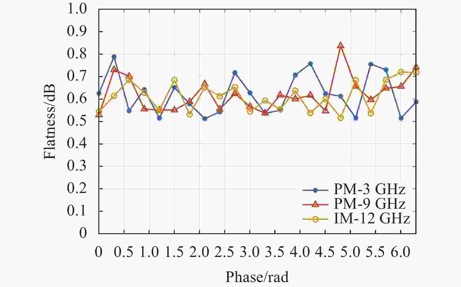

在不同的光学频率梳谱线根数要求下,遍历驱动相位调制器与强度调制器的谐波组合得到光学频率梳谱线根数与平坦度的关系,选取平坦度小于1 dB且谐波数量最少的微波驱动信号组合。如图12所示,当谱线根数不超过7时,平坦度为0 dB;当谱线根数大于7时,平坦度随着谱线根数的增加而增大。

图 12 光学频率梳谱线根数与平坦度的关系
Figure 12. Relationship between number of comb lines and flatness of the generated OFC
-
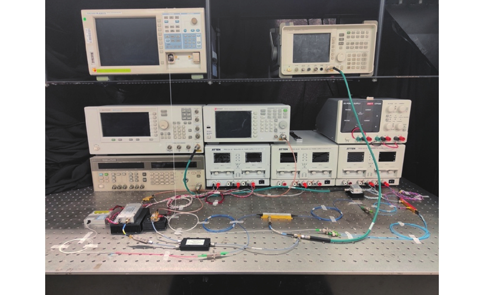
文中对图1所示产生平坦光学频率梳的方法进行了实验验证,以叠加的基频信号和三次谐波驱动相位调制器,以四次谐波驱动强度调制器,其中三次谐波的相位不作调谐。实验图如图13所示,具体实验过程如下。
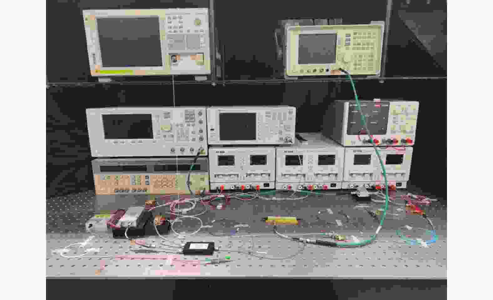
图 13 使用级联的相位调制器和强度调制器生成平坦光学频率梳的实验图
Figure 13. Experiment setup of the generation for flat optical frequency comb by using cascaded phase modulator and intensity modulator
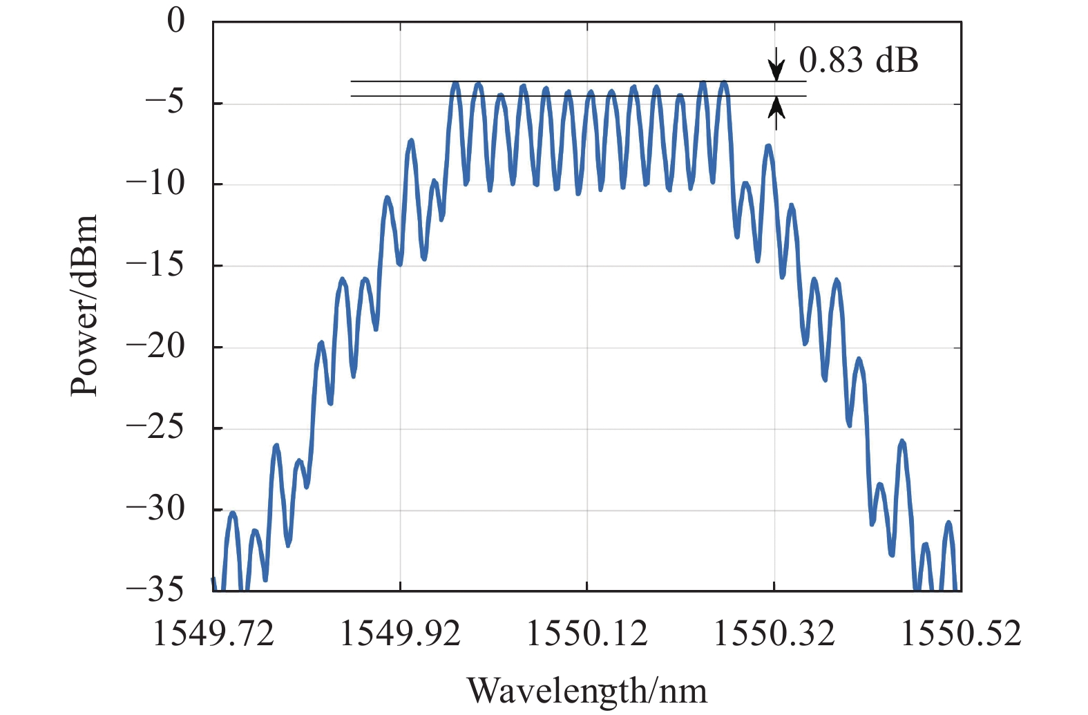
激光器(Han's Raypro Sensing RP-MR-C34-A0 B0-02-0)输出1550.12 nm的连续光,功率为16.78 dBm。该连续光经过相位调制器(iXblue MPZ-LN-40)被叠加到同步后的基频信号和三次谐波调制。基频信号(Keysight N9310A)频率为3 GHz,三次谐波(HP 83732A)频率为9 GHz。在合并之前,3 GHz基频信号依次经过移相器(phase shifter, PS)和放大器(amplifier, AMP),9 GHz谐波信号仅经过放大器。合并的基频信号和三次谐波驱动相位调制器,其功率分别为18.67 dBm和17.00 dBm。需要注意的是,为了抑制放大器非线性效应带来的谐波分量,在3 GHz基频信号所在支路的放大器后放置了带通滤波器。调相后的激光经过强度调制器(EOSPACE AX-1x2-0S5-10-PFA-PFA)。强度调制器的驱动信号为四次谐波(Agilent E8257D),频率为12 GHz,功率为20.50 dBm。四次谐波与之前的基频和三次谐波已同步。调节强度调制器的偏置电压和驱动信号的相位与幅度,在光谱仪(optical spectrum analyzer, OSA;型号Yokogawa AQ6370)上观察到平坦度为0.83 dB的13根谱线光学频率梳,如图14所示。所得到的实验图与图3所示的仿真图趋势一致。

图 14 光学频率梳实验图。基频、三次谐波驱动相位调制器,四次谐波驱动强度调制器
Figure 14. OFC in experiment, where the PM is driven by fundamental tone and third harmonic and the IM is driven by fourth harmonic
-
文中提出了一种产生平坦光学频率梳的方法。该方法让叠加的谐波驱动级联的相位调制器和强度调制器,通过调节相位调制器、强度调制器驱动信号的调制指数和相位以及强度调制器的偏置相位等参数,得到平坦的光学频率梳。文中以最小化光学频率梳各个频率分量功率方差为目标,使用差分进化算法得到相位调制器、强度调制器的各个优化参数。通过该方法,文中得到了产生平坦光学频率梳的驱动相位调制器和强度调制器的各种谐波组合。研究表明,当固定某一微波驱动信号的相位时,同样可以得到平坦的光学频率梳。这一现象经过了仿真和实验的验证。在实验中当基频和三次谐波驱动相位调制器、四次谐波驱动强度调制器,并且固定三次谐波的相位时,可以产生13根谱线、平坦度为0.83 dB的光学频率梳。实验结果符合仿真结果,证实了上述产生平坦光学频率梳方法的可行性和鲁棒性。
Approach to generation of flat optical frequency comb using cascaded phase modulator and intensity modulator
-
摘要: 光学频率梳在光通信、光谱学等领域有广泛的应用。平坦度是光学频率梳重要的性能指标。使用级联相位调制器和强度调制器产生光学频率梳的方法,是让叠加的谐波驱动调制器,通过调节驱动电信号的幅度和相位以及强度调制器的偏置电压,可以实现平坦度好的光学频率梳。首先,建立光学频率梳的优化问题模型,通过差分进化算法得到上述各个参数,并得到在不同叠加微波驱动信号下的平坦光学频率梳。其次,固定某一微波驱动信号的相位,在同一优化问题下使用同样方法得到微波驱动信号的其他参数,并分析生成的平坦光学频率梳性能。最后,搭建实验系统,根据仿真得到的优化参数确定实验参数,并得到相应的光学频率梳。研究表明,当采用基频和三次谐波驱动相位调制器、采用四次谐波驱动强度调制器时,可以产生13根谱线的光学频率梳,仿真和实验时的平坦度分别为0.27 dB和0.83 dB。当采用基频、三次谐波和五次谐波同时驱动相位调制器和强度调制器时,可以产生19根谱线的光学频率梳,仿真显示其平坦度为0.56 dB。以上仿真和实验结果证明了所提方法的可行性和鲁棒性。Abstract:
Objective Optical frequency comb (OFC) is widely used in optical communication system and spectroscopy. OFC can be generated by using mode-locked laser and electro-optic modulators (EOMs). Although the EOM-based OFC has good performance of flexibility, its flatness performance can be improved. The flatness of OFC is determined mainly by the modulation index and phase of driving microwave signal in phase modulation, which is the fundamental process of electro-optic modulation. Therefore, the optimized modulation index and phase of driving signal as well as other parameters are critical to the generation of flat OFC. In addition, due to the periodicity of driving signals' phases, one of the phases can be left without adjustment in the experiment to achieve flat OFC. However, to the best of the authors' knowledge, this phenomenon has seldom been investigated. Methods An approach to the generation of flat OFC is proposed, where cascaded phase modulator (PM) and intensity modulator (IM) are driven by combined harmonics (Fig.1). The parameters of driving harmonics and IM are optimized, where the optimization problem is formulated to minimize the variance of power for the OFC with certain number of comb lines. Differential evolution (DE) algorithm is applied to solve the optimization problem. Feasible solutions for combined harmonics are investigated in simulation. Experiment is also carried out to verify the feasibility of proposed approach (Fig.13). Although the phases of all the combined driving harmonics can be optimized, it is found that one of the driving harmonics' phases can be left without optimization while the performance of flatness is not affected. Results and Discussions When the fundamental tone and third harmonic are combined to drive the PM and the fourth harmonic drives the IM, a 13-line OFC is generated, where the flatness is 0.27 dB and 0.83 dB under simulation and experiment respectively (Fig.3, Fig.14). When the fundamental tone, third harmonic, and fifth harmonic are combined to drive both the PM and IM, a 19-line OFC with 0.56 dB flatness is achieved in simulation (Fig.4). The rest feasible solutions to generate flat OFC are listed (Tab.1). The relationship between number of comb lines and flatness is also investigated (Fig.12). When the number of comb lines is no larger than 7, the flatness is 0 dB; when the number of comb lines is larger than 7, the flatness increases as the number of comb lines grows. If the phase of one of the driving harmonics is fixed when the optimization problem is being solved, the flatness performances for the cases listed (Tab.1) are not affected (Fig.5, Fig.9-11). Regarding the case in Tab.1(b), the modulation indices for all the three driving harmonics are also investigated, when one of three harmonics' phases is fixed in the simulation (Fig.6-8). Conclusions This work investigates the approach to generate flat OFC by using cascaded PM and IM. These EOMs are driven by combined harmonics, where the parameters are optimized, such as the modulation index and phase of each driving harmonic as well as the bias phase caused by the bias voltage of IM. The optimized parameters are obtained by using DE algorithm, which solves the optimization problem to minimize the variance of power for the OFC. Both simulation and experiment have been carried out to achieve flat OFC. When the combined fundamental tone as well as third harmonic drive the PM and the fourth harmonic drives the IM, a 13-line OFC is generated with 0.27 dB and 0.83 dB flatness under simulation and experiment respectively. It is found that when one of the driving harmonics' phases is fixed, flat OFC can also be achieved by solving the same optimization problem. This phenomenon makes it possible to generate flat OFC in the experiment without adjusting that phase. Therefore, both the feasibility and robustness of the proposed approach are guaranteed. -
Key words:
- optical frequency comb /
- phase modulator /
- intensity modulator /
- combined harmonics
-
图 1 使用级联相位调制器和强度调制器产生平坦光学频率梳的方法
Figure 1. Schematic to generate flat OFC by using cascaded PM and IM
图 2 驱动相位调制器的叠加的基频和三次谐波波形
Figure 2. Waveform of combined fundamental tone and third harmonic that drive the PM
图 3 光学频率梳仿真图。基频、三次谐波驱动相位调制器,四次谐波驱动强度调制器
Figure 3. OFC in simulation, where the PM is driven by combined fundamental tone and third harmonic and the IM is driven by fourth harmonic
图 4 光学频率梳仿真图。基频、三次、五次谐波驱动相位调制器和强度调制器
Figure 4. OFC in simulation, where the combined fundamental tone, third and fifth harmonic drive both PM and IM
图 12 光学频率梳谱线根数与平坦度的关系
Figure 12. Relationship between number of comb lines and flatness of the generated OFC
图 13 使用级联的相位调制器和强度调制器生成平坦光学频率梳的实验图
Figure 13. Experiment setup of the generation for flat optical frequency comb by using cascaded phase modulator and intensity modulator
图 14 光学频率梳实验图。基频、三次谐波驱动相位调制器,四次谐波驱动强度调制器
Figure 14. OFC in experiment, where the PM is driven by fundamental tone and third harmonic and the IM is driven by fourth harmonic
表 1 产生平坦光学频率梳的叠加谐波组合
Table 1. Combinations of harmonics for the generation of flat OFC
Case Combined harmonics
that drive PMParameters of harmonics
that drive PMCombined harmonics
that drive IMParameters of harmonics
that drive IMNumber of
comb linesFlatness/dB (a) $ {f}_{0} $ ,$ 3{f}_{0} $ $ {\;\beta }_{\mathrm{P}\mathrm{M},1}= $ 1.50$ {\;\beta }_{\mathrm{P}\mathrm{M},3}= $ 1.20$ {\varphi }_{\mathrm{P}\mathrm{M},1}= $ 1.75$ {\varphi }_{\mathrm{P}\mathrm{M},3}= $ 5.93$ 2{f}_{0} $ $ {\;\beta }_{\mathrm{I}\mathrm{M},2}= $ 0.45$ {\varphi }_{\mathrm{I}\mathrm{M},2}= $ 3.05$ {\varphi }_{\mathrm{B}\mathrm{i}\mathrm{a}\mathrm{s}}= $ 3.239 0.59 (b) $ {f}_{0} $ ,$ 3{f}_{0} $ $ {\;\beta }_{\mathrm{P}\mathrm{M},1}= $ 1.48$ {\;\beta }_{\mathrm{P}\mathrm{M},3}= $ 1.12$ {\varphi }_{\mathrm{P}\mathrm{M},1}= $ 3.01$ {\varphi }_{\mathrm{P}\mathrm{M},3}= $ 3.85$ 4{f}_{0} $ $ {\;\beta }_{\mathrm{I}\mathrm{M},4}= $ 1.06$ {\varphi }_{\mathrm{I}\mathrm{M},4}= $ 3.09$ {\varphi }_{\mathrm{B}\mathrm{i}\mathrm{a}\mathrm{s}}= $ 2.9313 0.27 (c) $ {f}_{0} $ ,$ 3{f}_{0} $ $ {\;\beta }_{\mathrm{P}\mathrm{M},1}= $ 1.35$ {\;\beta }_{\mathrm{P}\mathrm{M},3}= $ 0.92$ {\varphi }_{\mathrm{P}\mathrm{M},1}= $ 3.32$ {\varphi }_{\mathrm{P}\mathrm{M},3}= $ 5.20$ {f}_{0} $ ,$ 3{f}_{0} $ ,$ 5{f}_{0} $ $ {\;\beta }_{\mathrm{I}\mathrm{M},1}= $ 0.97$ {\;\beta }_{\mathrm{I}\mathrm{M},3}= $ 0.63$ {\;\beta }_{\mathrm{I}\mathrm{M},5}= $ 1.01$ {\varphi }_{\mathrm{I}\mathrm{M},1}= $ 0.17$ {\varphi }_{\mathrm{I}\mathrm{M},3}= $ 6.10$ {\varphi }_{\mathrm{I}\mathrm{M},5}= $ 0.70$ {\varphi }_{\mathrm{B}\mathrm{i}\mathrm{a}\mathrm{s}}= $ 3.1317 0.45 (d) $ {f}_{0} $ ,$ 3{f}_{0} $ ,$ 5{f}_{0} $ $ {\;\beta }_{\mathrm{P}\mathrm{M},1}= $ 1.36$ {\;\beta }_{\mathrm{P}\mathrm{M},3}= $ 1.02$ {\;\beta }_{\mathrm{P}\mathrm{M},5}= $ 1.06$ {\varphi }_{\mathrm{P}\mathrm{M},1}= $ 4.34$ {\varphi }_{\mathrm{P}\mathrm{M},3}= $ 5.18$ {\varphi }_{\mathrm{P}\mathrm{M},5}= $ 2.44$ {f}_{0} $ ,$ 3{f}_{0} $ ,$ 5{f}_{0} $ $ {\;\beta }_{\mathrm{I}\mathrm{M},1}= $ 0.29$ {\;\beta }_{\mathrm{I}\mathrm{M},3}= $ 1.04$ {\;\beta }_{\mathrm{I}\mathrm{M},5}= $ 0.87$ {\varphi }_{\mathrm{I}\mathrm{M},1}= $ 5.82$ {\varphi }_{\mathrm{I}\mathrm{M},3}= $ 0.84$ {\varphi }_{\mathrm{I}\mathrm{M},5}= $ 0.80$ {\varphi }_{\mathrm{B}\mathrm{i}\mathrm{a}\mathrm{s}}= $ 0.0119 0.56  下载: 导出CSV
-
[1] Du Junting, Chang Bing, Li Zhaoyu, et al. Mid-infrared optical frequency combs: Progress and application (Invited) [J]. Infrared and Laser Engineering, 2022, 51(3): 20210969. (in Chinese) doi: 10.3788/IRLA20210969 [2] Liu Pengfei, Ren Linhao, Wen Hao, et al. Progress in integrated electro-optic frequency combs (Invited) [J]. Infrared and Laser Engineering, 2022, 51(5): 20220381. (in Chinese) doi: 10.3788/IRLA20220381 [3] Kayes M I, Rochette M. Precise distance measurement by a single electro-optic frequency comb [J]. IEEE Photonics Technology Letters, 2019, 31(10): 775-778. doi: 10.1109/LPT.2019.2907576 [4] Lundberg L, Mazur M, Mirani A, et al. Phase-coherent lightwave communications with frequency combs [J]. Nature Communications, 2020, 11(201): 1-7. [5] Parriaux A, Hammani K, Millot G. Electro-optic frequency combs [J]. Advances in Optics and Photonics, 2020, 12(1): 223-287. doi: 10.1364/AOP.382052 [6] Gheorma I L, Gopalakrishnan G K. Flat frequency comb generation with an integrated dual-parallel modulator [J]. IEEE Photonics Technology Letters, 2007, 19(13): 1011-1013. doi: 10.1109/LPT.2007.898766 [7] Chen C H, He C, Zhu D, et al. Generation of a flat optical frequency comb based on a cascaded polarization modulator and phase modulator [J]. Optics Letters, 2013, 38(16): 3137-3139. doi: 10.1364/OL.38.003137 [8] Wu R, Supradeepa V R, Long C M, et al. Generation of very flat optical frequency combs from continuous-wave lasers using cascaded intensity and phase modulators driven by tailored radio frequency waveforms [J]. Optics Letters, 2010, 35(19): 3234-3236. doi: 10.1364/OL.35.003234 [9] Li D, Wu S, Liu Y, et al. Flat optical frequency comb generation based on dual-parallel Mach-Zehnder modulator and a single recirculation frequency shift loop [J]. Applied Optics, 2020, 59(7): 1916-1923. doi: 10.1364/AO.381880 [10] Ozharar S, Quinlan F, Ozdur I, et al. Ultraflat optical comb generation by phase-only modulation of continuous-wave light [J]. IEEE Photonics Technology Letters, 2008, 20(1): 36-38. doi: 10.1109/LPT.2007.910755 [11] Wang Q, Huo L, Xing Y F, et al. Ultra-flat optical frequency comb generator using a single-driven dual-parallel Mach-Zehnder modulator [J]. Optics Letters, 2014, 39(10): 3050-3053. doi: 10.1364/OL.39.003050 [12] Lin T, Zhao S H, Zhu Z H, et al. Generation of flat optical frequency comb based on a DP-QPSK modulator [J]. IEEE Photonics Technology Letters, 2017, 29(1): 146-149. doi: 10.1109/LPT.2016.2630313 [13] Qu K, Zhao S H, Li X, et al. Ultra-flat and broadband optical frequency comb generator via a single Mach–Zehnder modulator [J]. IEEE Photonics Technology Letters, 2017, 29(2): 255-258. doi: 10.1109/LPT.2016.2640276 [14] Dou Y J, Zhang H M, Yao M Y. Generation of flat optical-frequency comb using cascaded intensity and phase modulators [J]. IEEE Photonics Technology Letters, 2012, 24(9): 727-729. [15] Cui Y H, Wang Z X, Xu Y T, et al. Generation of flat optical frequency comb using cascaded PMs with combined harmonics [J]. IEEE Photonics Technology Letters, 2022, 34(9): 490-493. doi: 10.1109/LPT.2022.3168378 [16] Chi H, Zou X H, Yao J P. Analytical models for phase-modulation-based microwave photonic systems with phase modulation to intensity modulation conversion using a dispersive device [J]. Journal of Lightwave Technology, 2009, 27(5): 511-521. doi: 10.1109/JLT.2008.2004595 [17] 周炯槃. 通信原理 [M]. 北京: 北京邮电大学出版社, 2008. [18] 王文婕. 天线阵列二维波达方向估计算法研究[D]. 北京: 北京邮电大学, 2018 Wang Wenjie. Research on two-dimensional direction of arrival estimation algorithms for the antenna array[D]. Beijing: Beijing University of Posts and Telecommunications, 2018. (in Chinese) [19] Weber H, Arfken G. Essential Mathematical Methods for Physicists [M]. San Diego: Elsevier, 2004. [20] Feoktistov V. Differential Evolution-In Search of Solutions [M]. New York: Springer, 2006. -

 点击查看大图

计量
- 文章访问数: 248
- HTML全文浏览量: 49
- PDF下载量: 46
- 被引次数: 0


