


-
随着遥感相机更大幅宽和更高灵敏的探测需求,相机一般需要大视场和大口径的配置。大口径光学系统为了扩大成像幅宽,通常会采用扫描的方式来实现[1-4]。大口径光学系统的扫描镜为平面镜,在主光学系统光路的最前端,通过转动扫描镜将不同角度的入射光折转入主光路,以实现扩大相机视场的目标。
遥感相机受限于有限的空间约束,系统的遮光罩长度受限,同时系统的功耗和质量也限制了遥感相机的热控能力。因此,作为光学系统中的第一个光学组件,容易暴露在太阳辐射和地球反照之下,也容易受到相机自身结构件辐射的影响,如遮光罩、蒙皮板等,都会使得反射镜的温度场发生改变,产生的热应力会导致反射镜面型变化,进一步影响到相机的成像质量,限制相机在轨的可用时间[5-7]。
为了规避由于外热流导致的反射镜面型变化,一般会采用反射镜转向规避或平台机动规避等方法,此类方法会损失遥感相机的在轨可用时间。为了尽可能减少相机可用时间的损失,可以采用波前补偿的方式来实现对于镜面面型变化的补偿。补偿光学系统的波前需要首先测量出光学系统的波前变化,以此变化为基础改变相应光学元件的面型从而实现对于波前的补偿。通常,测量光学系统的波前变化需要采用波前传感器[8-9],此类方法目前在遥感相机研制上并不被经常使用,主要原因是在光学系统中需要增加波前测试光路、波前传感器以及相应的辅助组件,带来了质量、功耗以及空间的额外需求,且对于大口径相机无法实现全光路的探测,一般只针对局部孔径进行测试,具有局限性。
文中提出的测试方法是基于算法结合干涉仪和反射镜背部测温,所建立的反射镜温度场与反射镜镜面形变间的关系模型。通过验证,该方法可实现优于RMS 1/50λ(λ=0.6328 µm)的面型还原精度。其核心是如何建立反射镜温度场与面型变化间的关系,为此文中提出了以反射镜背部测温点为依据,利用神经网络算法[10]反演出反射镜的面型变化,从而为后光路使用变形镜进行校正提供依据[11]。该方法无需增加额外波前测试系统,减小光学系统的实现难度以及质量、功耗等额外的载荷负担,更有利于在轨应用。
-
遥感相机的扫描镜在轨应用时需要进行频繁的摆动,且需要实现较高的控制精度,测温点、加热片的引线也容易对扫描镜的在轨适用性产生影响。受限于在轨遥感相机的温控资源,以及反射镜控制可靠性的要求,反射镜的测、控温数量会保留最低的需求数量,且测、控温点需要贴在反射镜的背部。文中的目标是在不使用高精度波前测试系统的情况下,通过反射镜背部有限的测温点,反演出扫描镜表面的面型变化。
当反射镜受到外热流影响时,镜面会产生温度梯度,从而改变现有面型。为解算出两者的关系,可以将反射镜测温点的温度变化与其面型变化间建立数学表达式:
$$ \Delta W=f\left(\Delta {T}_{1},\Delta {T}_{2},\cdots, \Delta {T}_{n}\right) $$ (1) 式中:∆W表示反射镜的面型变化量;∆Ti(i=1~n)为n个测试点的温度值变化。由于反射镜的温度场变化主要来源于外热流和相机蒙皮或结构温度变化导致的辐射变化,因此各个测温点间的温度场关系具有关联性,可以排除部分点温度突变的情况。建立面型变化量与背部温度值变化的准确数学表达较为困难,因此可以采用神经网络的算法,通过多工况的训练,得出温度与面型变化的关系,如此能够极大降低算法复杂性带来的计算误差,并可以充分利用神经网络的泛化性有效抑制噪声对计算结果的影响。
反射镜的面型变化∆W可以用多种方式表示,包括反射镜表面的点云、或者面型数值拟合。采用点云的表述方式能较为准确地将面型的细节变化表现出来,但数据量较大,相对于有限的测温点,面型点云表达将对算法迭代增加计算难度,因此采用面型的数值拟合方式对面型变化进行表达。文中采用了Zernike多项式对反射镜面型进行表示。Zernike多项式[12]数学表达式为:
$$ Z\left(r,\theta \right)=\sum _{n}\sum _{m}\left[{A}_{nm}{P}_{nm}\left(\rho \right)\mathrm{cos}\left(m\theta \right){+B}_{nm}{P}_{nm}\left(\rho \right)\mathrm{sin}\left(m\theta \right)\right] $$ (2) 其中
$$ {P}_{nm}\left(\rho \right)=\sum\nolimits _{j=0}^{\tfrac{n-m}{2}}C\left(n,m,j\right){\rho }^{n-2j} $$ (3) $$ C\left(n,m,j\right)=\frac{{\left(-1\right)}^{j}\left(n-j\right)!}{j!\left(({n+m})/{2}-j\right)!\left(({n+m})/{2}-j\right)!} $$ (4) 式中:ρ为镜面半径的归一化值;n和m为多项式的角向级数和径向级数,可以根据拟合面型精度的需求进行调整。Zernike多项式的不同项代表反射镜不同的像差的变化。因此,为了通过反射镜背部温度点反演出反射镜的面型变化,等价于计算出通过各测温点温度变化解算出Zernike多项式各像差参数的变化。文中提出使用神经网络算法通过所测量反射镜背部的测温点温度变化反向解算出反射镜面型变化情况,如此便能够根据反射镜的面型变化指导后续光路的波前补偿方案。
-
利用BP神经网络算法根据反射镜背部有限的测温点温度变化情况反演反射镜的面型变化,需要建立一套以有限元分析结果为基础的温度与面型变化的模型。
算法流程见图1。具体步骤分解如下:

图 1 分析模型构建方法的流程图
Figure 1. The flow chart of the construction of analysis model
Step1:
利用三反系统作为分析模型,如图2所示。
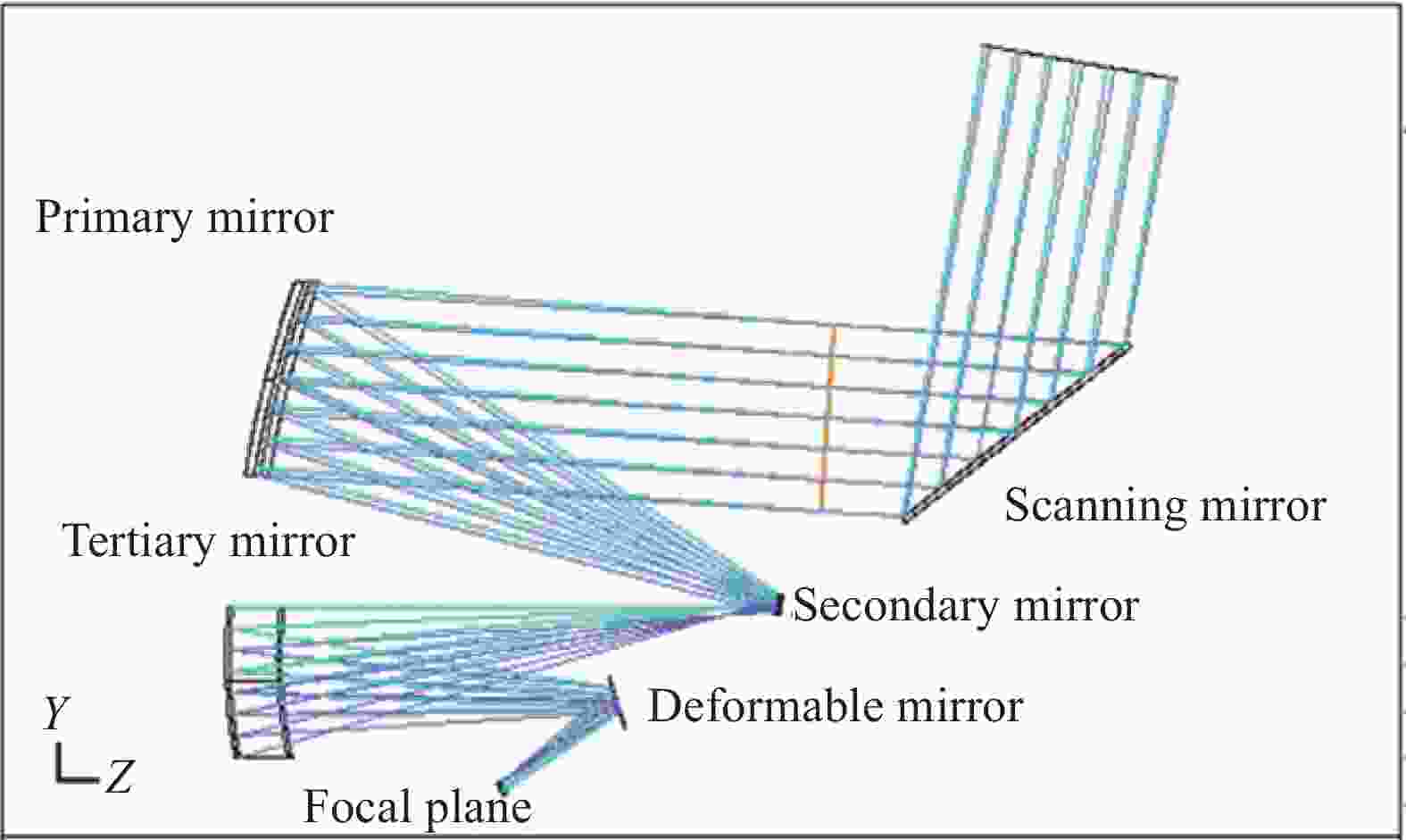
图 2 三反成像光学系统的光路图
Figure 2. Optical path diagram of three mirror optical system layout
首先,建立遥感相机的光学与结构模型,遥感相机的光学参数见表1。相机的扫描镜位于相机的最前端入光口处,受到太阳、地球辐照的影响较大,为减小反射镜所受到外热流影响,反射镜通常采用如SiC、ULE或Zerodur等材料,相对于ULE、Zerodur材料,SiC具有更好的比刚度,可以获得较好的轻量化效果。该相机的扫描镜采用了SiC材料,具体的参数值如表2所示。
表 1 光学系统参数表
Table 1. Parameters of the optical system
No. Parameter Value 1 Field of view/(°) 1.0×4.0 2 Aperture/nm φ120 3 Wavelength/µm 0.55-0.90 4 Focal length 350 表 2 SiC材料的关键参数值
Table 2. The key parameters of SiC
No. Parameter Value 1 Density/kg·m−3 3.1 2 Young’s modulus/GPa 403 3 Poisson’s ratio 0.168 4 Isotropic instantaneous coefficient of
thermal expansion/×10−6 K2.24 5 Isotropic thermal conductivity λ/W·m·K−1 140 扫描镜的尺寸为200 mm×140 mm的近似椭圆形,经过轻量化后的结构形状如图3所示。

图 3 扫描镜轻量化结构图
Figure 3. Lightweight structure of scanning mirror
Step2:
反射镜的热弹变化主要来自于载荷在轨的外热流影响以及反射镜周围组件的热辐射。为了建立反射镜背部测温点温度变化和反射镜面型变化的关系,可以将热分析结果中的极值工况作为分析范围,在极值范围内随机选取n种工况为神经网络算法的数据输入,对应分析这些情况下反射镜相应的面型变化,随后将反射镜的面型变化换算成Zernike多项式的表达式。
Step3:
反射镜的面型可以用Zernike多项式进行表达。选取的Zernike阶数越高(公式(2)中的n和m),反射镜面型的拟合精度越高。但由于神经网络算法的收敛特性,Zernike系数的个数应不多于测温点的个数。反射镜测温点的个数受限于星上资源、运动可靠性等因素,通常较为少量,因此测温点的选取直接决定了Zernike多项式拟合系数个数的选取。可以在满足Zernike拟合精度的前提下,选取最少的多项式参数数量,从而对应不小于该数量的测温点数量。Zernike多项式所对应的面型像差见表3,表中$ \theta $为极坐标角度,$ \; \rho $为半径。
表 3 Zernike 多项式前11项表达式及对应的像差含义
Table 3. The meaning of the first 11 terms of Zernike polynomial
n m Term Polynomial Meaning 0 0 0 1 Piston 1 +1 1 $ \rho \mathrm{cos}\theta $ Tilt X 1 −1 2 $ \rho \mathrm{sin}\theta $ Tilt Y 1 0 3 $ 2\;{\rho }^{2}-1 $ Power 2 +2 4 $ \;{\rho }^{2}\mathrm{cos}2\theta $ Astigmatism X 2 −2 5 $ \;{\rho }^{2}\mathrm{sin}2\theta $ Astigmatism Y 2 +1 6 $ \left(3\;{\rho }^{2}-2\right)\rho \mathrm{cos}\theta $ Coma X 2 −1 7 $ \left(3\;{\rho }^{2}-2\right)\rho \mathrm{sin}\theta $ Coma Y 2 0 8 $ 6\;{\rho }^{4}-6\;{\rho }^{2}+1 $ Primary spherical 3 +3 9 $ \;{\rho }^{3}\mathrm{cos}3\theta $ Trefoil X 3 −3 10 $ \;{\rho }^{3}\mathrm{sin}3\theta $ Trefoil Y 由于入射光为平行光,因此一阶像差中平移、倾斜不会对相机像质产生影响,而彗差、像散、球差、三叶草像差则是需要进行校正的像差,离焦量对于平面反射镜是相当关键的像差,通常会产生像面的离焦,需要通过调焦机构进行补偿[13]。在进行BP神经网络的计算时,平移、倾斜像差可以忽略,同时将各个像差转换成极坐标的表达方式,如此可以针对特定像差的幅度或方向属性进行权重的修改,有利于算法的收敛。
Step4:
建立BP神经网络需要将反射镜背部测温点的温度变化数据作为神经网络的输入层,每个测温数据对应一个输入节点。将反射镜面型转换为Zernike多项式参数后,将各像差所对应的Zernike多项式的系数作为BP神经网络的输出层数据,每个系数对应一个输出节点。如图4所示 。

图 4 BP神经网络构成图
Figure 4. The diagram of BP neural network
通过多个工况下的温度值与面型Zernike参数值训练,可以得出最终的BP神经网络各级的权重值模型。建立BP神经网络算法的流程图见图5。

图 5 人工神经网络算法流程图
Figure 5. The flow chart of artificial BP network algorithm
S1:初始化各个参数,设置计算轮为N=200,并且归一化输入参数。输入值为反射镜背部的测温点数据,n个测温点的温度值为$ { {{T_1}}, \cdots ,{{T_n}} } $,可以使用公式(5)将每个温度点的温度值进行归一化:
$$ \operatorname{Norm}\left(T_i\right)=\left(T_i-\dfrac{\displaystyle \sum\nolimits_{i=1}^n T_i}{n}\right) \Biggr/ \max _n\left(\left|T_1, \cdots, T_n\right|\right) $$ (5) 式中:归一化的第i个测温点温度值Norm(Ti)等于Ti减去所有测温点的平均温度值除以所有测温点温度绝对值的最大值。
S2:首先产生一组随机的权重值$ {\omega }_{ij} $,随机权重值为输入层与隐藏层间的权重,权重的选取范围为−1<$ {\omega }_{ij} $<1。隐藏层与输出层间的权重$ {v}_{jk} $,同理权重的选取范围为−1<$ {v}_{jk} $<1。
S3:通过输入层与隐藏层之间的权重计算隐藏层的输出值,可表示为:
$$ {O}_{H}={\rm{sigmoid}}\left({W}_{I-H} \cdot I\right) $$ (6) 式中:I表示输入层的矩阵,为镜面的测温点的温度值;$ {W}_{I-H} $为输入层与隐藏层间的权重值矩阵;$ {\omega }_{ij}\in {W}_{I-H} $;$ {O}_{H} $为隐藏层的输出值矩阵;Sigmoid为S型生长曲线。
S4:通过隐藏层与输出层之间的权重计算输出层的输出值为:
$$ {O}_{O}={\rm{sigmoid}}\left({V}_{H-O} \cdot {O}_{H}\right) $$ (7) 式中:$ {O}_{H} $表示隐藏层的输出矩阵;$ {V}_{H-O} $为隐藏层与输出层间的权重矩阵;$ {v}_{jk}\in {V}_{H-O} $、$ {O}_{H} $为隐藏层的输出值矩阵。
S5:比较输出层的输出值与期望值间的差值,可以得出此轮计算后的模型误差。由于每种像差对最终的成像质量影响不同,且部分的像差可以通过后期算法进行残差的消除[13],因此针对输出值权重可以设置不同值。输出层误差可以表示为各个节点的误差的平方和,通过对输出值节点的权重设置,每个输出节点的输出值与期望值间的误差平方后乘上该节点的权重,然后求和。总输出误差$ {E}_{o} $可以表示为:
$$ {E}_{o}=\sum\nolimits _{{k}=1}^{{n}}{q}_{{k}} \cdot {\left({o}_{{k}}-{a}_{{k}}\right)}^{2} $$ (8) 式中:$ {q}_{{k}} $为第k个输出节点的权重;$ {o}_{{k}} $为第k个输出节点的数值;$ {a}_{{k}} $为第k个输出节点的期望值。
S6:每轮计算完成后需要判断当前计算轮是否已经结束,同时选用判断输出的误差值是否小于等于阈值Th,此处阈值可以选取接近于0的值,如10−5。
S7:S6的判断为错误时,需要更新权重值,输出层与隐藏层之间的权重更新的方式为:
$$ {v}_{j,k}^{{'}}={v}_{j,k}-\alpha \cdot \frac{\partial {E}_{o}}{\partial {v}_{j,k}} $$ (9) 式中:$ {v}_{{j},{k}}^{{{'}}} $为更新后的权重值;$ {v}_{{j},{k}} $为更新前的权重值;式中的下标j为隐藏层的节点编号;k为对应输出层的节点号; $ \alpha $为学习率,初始值可设为0.01;$\partial {E}_{{o}} / \partial {y} $为误差函数相对于权重值变化的斜率。斜率可表示为:
$$ \frac{\partial {E}_{o}}{\partial {v}_{{j},{k}}}=\frac{\partial {E}_{o}}{\partial {O}_{k}} \cdot \frac{\partial {O}_{k}}{\partial {v}_{{j},{k}}} $$ (10) $$\begin{split} \frac{\partial {E}_{o}}{\partial {v}_{{j},{k}}} = & -2\left({a}_{k}-{o}_{k}\right)\times {\rm{sigmoid}}\left({\sum }_{j}{v}_{{j},{k}} \cdot {h}_{{j}}\right) \cdot \\& \left(1-\left({\rm{sigmoid}}\left({\sum }_{j}{v}_{{j},{k}}\cdot {h}_{{j}}\right)\right)\right) \cdot {h}_{{j}} \end{split}$$ (11) 式中:$ {a}_{k} $为输出节点期望值;$ {o}_{k} $为节点的输出值;$ {h}_{{j}} $为隐藏层j节点的输出值。
同时需要更新输入层与输出层间的权重:
$$ \frac{\partial {E}_{o}}{\partial {\omega }_{{i},{j}}}=\frac{\partial {E}_{o}}{\partial {o}_{k}} \cdot \frac{\partial {o}_{{k}}}{\partial {h}_{{j}}} \cdot \frac{\partial {h}_{{j}}}{\partial {\omega }_{{i},{j}}} $$ (12) 式中:$ {\omega }_{{i},{j}} $为输入层与隐藏层间的权重值;i表示输入层第i个节点;j为隐藏层第j个节点。
同理,可得:
$$ \begin{split} \frac{\partial {E}_{o}}{\partial {\omega }_{{i},{j}}}= & {\sum }_{{k}}-2\left({a}_{{k}}-{o}_{{k}}\right)\times {\rm{sigmoid}}\left({\sum }_{j}{v}_{{j},{k}} \cdot {h}_{j}\right) \cdot \\& \left(1-\left({\rm{sigmoid}}\left({\sum }_{j}{v}_{{j},{k}} \cdot {h}_{{j}}\right)\right)\right)\times {\sum }_{{j}}{v}_{{j},{k}}\times \\& {\rm{sigmoid}}\left({\sum }_{{i}}{\omega }_{{i},{j}} \cdot {i}_{{i}}\right) \cdot \left(1-\left({\rm{sigmoid}}\left({\sum }_{{i}}{\omega }_{{i},{j}} \cdot {i}_{{i}}\right)\right)\right) \cdot {i}_{{i}} \end{split}$$ (13) 式中:$ {i}_{{i}} $为输入层i节点的输入值。输入层与隐藏层间的权重修正可表示为:
$$ {\omega }_{{i},{j}}^{{'}}={\omega }_{{i},{j}}-\alpha \cdot \frac{\partial {E}_{o}}{\partial {\omega }_{{i},{j}}} $$ (14) 然后回到S3,重新计算模型。
S8:S6的判断为正确时,接受权重模型。
Step5:
利用Step4便得出的BP神经网络权重值模型,如此便可以根据反射镜测温点数据反演出反射镜面型的变化情况。
-
为了验证该方法的有效性,采用一套离轴三反遥感相机模型进行验证,该模型的光路见图2,其结构如图6所示。
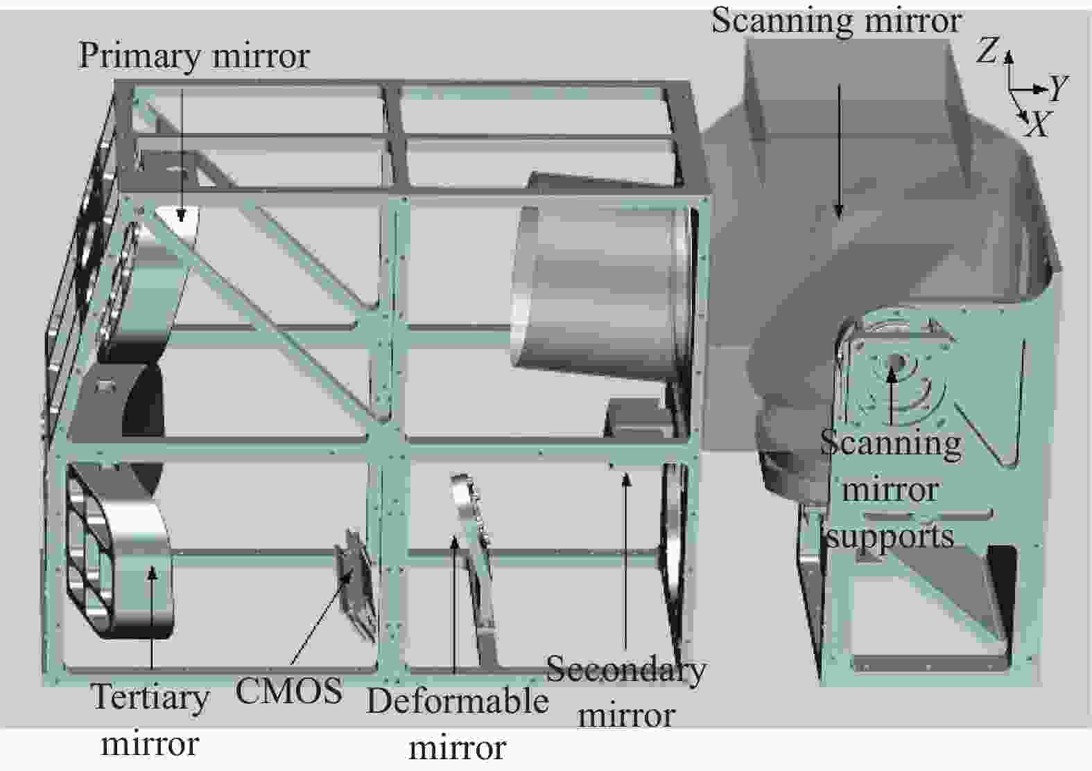
图 6 离轴三反遥感相机结构示意图
Figure 6. Structural schematic diagram of off-axis three mirror remote sensing camera
三反遥感相机采用了扫描镜进行扫描成像,扫描镜的支撑方式为两侧的穿轴安装,使其可以绕X轴进行转动,从而实现大视场成像。扫描镜由于处在整个光学系统最前端,且受限于整星的包络限制,相机的遮光罩长度有限,扫描镜相对于其他光学组件及结构件所受到在轨外热流的影响更大,扫描镜更加容易发生形变,从而导致相机成像质量的下降。根据分析在轨环境,可以通过有限元分析计算出不同工况下的扫描镜温度场变化和面型变化情况。
图7为遥感相机扫描镜和遮光罩的结构形式,在温度工况分析时除设置外热流-太阳和地球反照辐射外,还需将不同的温度工况赋值到遮光罩上,综合计算出扫描镜的温度变化。
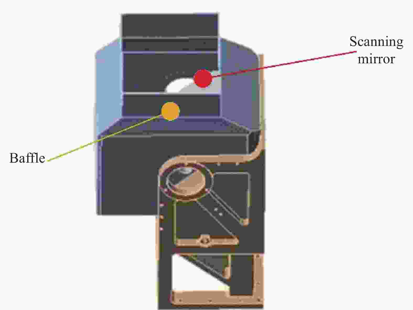
图 7 遥感相机扫的描镜与遮光罩的结构
Figure 7. Structure of the scanning mirror and light shield for remote sensing cameras
由于受限于在轨资源以及考虑到运动部件的可靠性,扫描镜的测温点需要贴在背部,且测温点数量也有限。在扫描镜的背部选取了8个测温点,测温点的分布情况如图8所示。

图 8 扫描镜背部测温点位置
Figure 8. Temperature measuring point on the back of scanning mirror
采用205套随机在轨外热流工况计算出扫描镜背部测温点的温度值以及所对应的反射镜面型变化情况,其中200套用于优化神经网络,剩余5套用于验证其有效性。在实际地面测试中,也可采用干涉仪在温度循环试验中测试扫描镜的面型变化,从而建立扫描镜测温点与反射镜面型变化间的多工况样本,用于训练神经网络模型。
将反射镜的面型变化转换为Zernike多项式的表达方式,选取面型中的彗差、像散、球差等8项主要影响最终成像面型的低阶像差,结合扫描镜背部8个测温点的温度值输入BP神经网络。BP神经网络采用3层结构,分别为输入层、隐藏层和输出层,输入层的节点数为8,8个测温点对应于输入层的8个节点,输出层节点数也为8,对应于Zernike多项式的8个参数,隐藏层采用16个节点。
其中,输出总误差算式中的权重用于对不同像差输出值进行权重调节, 8类像差中,如Power、Spherical、Trefoil等是难以利用后续图像算法进行校正的[13],因此可以采用较高的权重。相对地,Coma和Astigmatism则是可以通过后续图像算法进行校正,因此权重相对小。同时相对于像差的量级,像差的角度更加敏感,因此Coma、Astigmatism和Trefoil的角度值相对于幅度的权重更大。权重值可以根据每轮的测试结果进行调整,使得计算出的误差值最小。
BP神经网络的学习率α为一个可变量,可以根据输出的误差值进行调整,初始设置为0.01。设置阈值为Th=10−6。为了验证算法的有效性,用5种不同的随机外热流工况作为测试工况对算法进行测试,通过集成分析计算出扫描镜背部8个测温点的温度值,把温度值作为BP算法的输入值,可以计算出反射镜表面形变量的Zernike多项式的 系数值。表4为5种测试工况下,扫描镜背部8个测温点的温度情况。
表 4 扫描镜背部8个测温点的温度值(单位:℃)
Table 4. Temperature values of 8 temperature measurement points on the back of scanning mirror (Unit: ℃)
No. T1 T2 T3 T4 T5 T6 T7 T8 Ave temp 1 7.49 9.12 10.41 11.26 4.91 3.17 7.95 6.82 7.64 2 16.98 21.08 −0.2 5.14 19.66 17.05 8.26 5.58 11.69 3 22.90 20.87 2.6 1.44 21.12 22.82 7.49 9.24 13.56 4 18.87 14.05 9.62 5.58 16.93 19.89 10.75 13.88 13.70 5 24.29 21.38 17.12 14.63 24.39 26.38 19.45 21.33 21.12 将5种不同工况下的测温点值输入到BP神经网络中,可以计算出不同工况下的扫描镜面型的Zernike多项式像差系数值,如表5所示。
表 5 扫描镜面型Zernike多项式的像差系数
Table 5. Aberration coefficients of scanning mirror via Zernike polynomials
No. Power/λ Ast ρ/λ Ast θ/(°) Com ρ/λ Com θ/(°) Tref ρ/λ Tref θ/(°) Sph/λ 1 0.0330 0.0569 81.912 0.0603 68.336 0.0926 29.651 0.0379 2 0.0012 0.0326 40.045 0.0353 106.58 0.0801 28.686 0.0255 3 −5e-4 0.01395 32.6296 0.02962 59.6132 0.06413 37.1308 0.01664 4 −0.0024 −0.0036 93.065 0.0346 90.018 0.0503 39.795 0.0189 5 −0.018 0.0163 3.5802 0.00142 33.143 0.01940 9.2916 0.00100 通过比较扫描镜的温度工况相对于系统初始装调环境(20 ℃),温度场的变化范围跨度较大时,表4在工况1,温度的平均值为7.64 ℃,与常温环境的温差为12.36 ℃,大于其他4个工况的温度平均值,因此产生了更大的面型变化,而工况5的平均温度值与初始装调环境相近,面型变化较小。由此可见,扫描镜的面型变化不仅与扫描镜的温度均匀性有关,也与扫描镜的在轨温度相对于装调温度的温差有关。
通过对比有限元求解的反射镜理论面型变化与BP网络算法计算出面型变化验证该算法的有效性。如表6所示,通过两种方法所计算出的反射镜面型变化,相减后得出残差。表中,第一列为通过有限元分析得出的面型变化情况,第二列为通过BP神经网络算法计算出的面型变化,第三列则为两者相减的面型残差。
表 6 神经网络方法计算出的反射镜面型与理论面型的区别,λ=0.6328 µm
Table 6. The difference between the surface deformation calculated by neural network and the theoretical surface deformation, λ=0.632 8 µm
No. Theoretical surface deformation (RMS, λ) BP network algorithm (RMS, λ) Residual errors
(RMS, λ)1 0.049559 0.049555 0.0160 2 0.029358 0.035631 0.0195 3 0.022354 0.026707 0.0119 4 0.031312 0.024892 0.0133 5 0.012395 0.013173 0.0077 根据计算结果,通过神经网路计算出的面型与理论面型间的误差小于RMS 1/50λ(λ=0.6328 µm),约12.6 nm,可以满足扫描镜的面型公差要求。
图9中,波长λ为0.6328 µm,根据仿真计算结果可知,通过对随机的5个工况下扫描镜温度值的分析,可以正确地得出随温度场变化下的扫描镜面型变化。以此计算出的反射镜面型变化可以对调整后光路的变形镜进行面型补偿,从而实现相机成像质量的提升。

图 9 (a)、 (d)、 (g)、 (j) 、(m) 通过有限元分析计算出的扫描镜理论面型变化;(b)、 (e) 、(h) 、(k)、(n) BP神经网络算法计算出的面型变化;(c)、 (f)、 (i)、 (l)、 (o) 两者相减后的残差
Figure 9. (a), (d), (g), (j), (m) Theoretical surface deformation of the scanning mirror calculated by the finite element analysis; (b), (e), (h), (k), (n) Surface deformation calculated via BP network algorithm; (c), (f), (i), (l), (o) Residual errors
-
遥感相机扫描镜在外热流的影响下会对成像质量产生较大的影响,为了在轨能实现更为高效的成像补偿,文中提出了利用神经网络算法,通过扫描镜本身的测温点反演扫描镜面型的方法。通过该方法能够准确反演出扫描镜受到外热流产生的面型变化,进而为实现在后光路的补偿提供准确的面型值。通过仿真分析,该方法反演的面型变化与理论面型变化相差小于12.6 nm,为遥感相机在轨能够实现较好的面型测试、用于补偿外热流影响提供了新的解决方案。
Method for retrieving thermal deformation of scanning mirror of remote sensing camera via the neural network algorithm
-
摘要: 遥感相机的扫描镜通常位于光学系统的最前端,容易受到在轨外热流的影响产生非规则的面型变化,进而影响相机的成像质量。针对该问题设计了基于扫描镜温度值,以神经网络算法为基本,通过温度场变化反演扫描镜面型变化的扫描镜热变形测试方法。以该方法得出的扫描镜的面型变化可以作为后续成像系统面型修正的依据。该方法能够有效地提升遥感相机在轨的温度适用性,延长遥感相机的可用时间。通过该方法计算出的面型变化与理论面型变化的差值优于RMS 12.6 nm,具有较高的面型还原精度,验证了通过扫描镜温度值变化反演其面型变化的可行性。Abstract:
Objective Wide-range and high-resolution imaging is one of the important development directions of remote sensing cameras. In order to achieve wide-range and high-resolution imaging, the most common method is to scan a large field of view through a scanning mirror. As an important component of remote sensing cameras to achieve large field of view imaging, scanning mirrors are usually located at the forefront of the entire imaging system, and expand the imaging field of view by changing the incident optical angle. It is easily to expose the scanning mirror to the direct influence of external heat flow, such as sunlight and Earth's reflected light, which may lead to change in the temperature of the scanning mirror, and the thermal stress can lead to change in the surface figure of the scanning mirror, thereby affecting the imaging quality of the camera and limiting the available time of the camera in orbit. Therefore, when more resources cannot be provided to ensure the temperature stability of the scanning mirror, the best way to achieve high-quality imaging is to compensate for surface change caused by thermal deformation. How to accurately test the surface change of the scanning mirror in orbit becomes a key step in whether to compensate for thermal deformation surface change. Methods The proposed method is based on an algorithm that combines the interferometer data and the temperature of the mirror to establish a relationship model between the temperature of the mirror and the deformation of the mirror surface. In this paper, a neural network algorithm is adopted, which puts the temperature measurement values of the mirror as the input and the surface figure change of the mirror as the output (Fig.4). The function of inverting the surface mirror change of the mirror through the temperature values of the mirror can be realized. The input temperature values are provided by eight temperature measuring points on the back of the mirror (Fig.7). The surface figure of the mirror is expressed using a Zernike expression, including Power, Astigmatism, Coma, Trefoil, and Spherical aberration (Tab.5). Results and Discussions The method can achieve better performance than RMS 12.6 nm (Fig.8), which is a good performance. The core of the algorithm is how to establish the relationship between the temperature of the mirror and the surface figure change. Therefore, this paper proposes to use the neural network algorithm to reverse the surface figure change of the mirror based on the temperature measurement points on the back of the mirror, providing a basis for the use of deformable mirror in the rear optical path for correction. This method eliminates the need for additional wavefront testing systems, which can reduce the implementation difficulty of optical systems, as well as additional load burdens such as weight and power consumption. And The method is also more conducive to in-orbit applications. Conclusions The scanning mirror of a remote sensing camera has a significant impact on the imaging quality under the influence of external heat flow. In order to achieve more efficient imaging compensation in orbit, this paper proposes a method of using neural network algorithms to invert the surface figure change of the scanning mirror through the temperature measurement points of the scanning mirror itself. The method can accurately reflect the surface figure change of the scanning mirror caused by external heat flow, thereby providing accurate surface figure change for the compensation of the optical path after implementation. Through analysis, The residual errors between the retrieved surface figure and the theoretical surface figure is less than 12.6 nm, providing a new solution for remote sensing cameras to achieve better surface figure test method in orbit and to compensate for the impact of external heat flow. -
Key words:
- space optics /
- thermal stress analysis /
- image analysis /
- neural network algorithm
-
图 6 离轴三反遥感相机结构示意图
Figure 6. Structural schematic diagram of off-axis three mirror remote sensing camera
图 7 遥感相机扫的描镜与遮光罩的结构
Figure 7. Structure of the scanning mirror and light shield for remote sensing cameras
图 9 (a)、 (d)、 (g)、 (j) 、(m) 通过有限元分析计算出的扫描镜理论面型变化;(b)、 (e) 、(h) 、(k)、(n) BP神经网络算法计算出的面型变化;(c)、 (f)、 (i)、 (l)、 (o) 两者相减后的残差
Figure 9. (a), (d), (g), (j), (m) Theoretical surface deformation of the scanning mirror calculated by the finite element analysis; (b), (e), (h), (k), (n) Surface deformation calculated via BP network algorithm; (c), (f), (i), (l), (o) Residual errors
表 1 光学系统参数表
Table 1. Parameters of the optical system
No. Parameter Value 1 Field of view/(°) 1.0×4.0 2 Aperture/nm φ120 3 Wavelength/µm 0.55-0.90 4 Focal length 350  下载: 导出CSV
表 2 SiC材料的关键参数值
Table 2. The key parameters of SiC
No. Parameter Value 1 Density/kg·m−3 3.1 2 Young’s modulus/GPa 403 3 Poisson’s ratio 0.168 4 Isotropic instantaneous coefficient of
thermal expansion/×10−6 K2.24 5 Isotropic thermal conductivity λ/W·m·K−1 140
下载: 导出CSV
表 3 Zernike 多项式前11项表达式及对应的像差含义
Table 3. The meaning of the first 11 terms of Zernike polynomial
n m Term Polynomial Meaning 0 0 0 1 Piston 1 +1 1 $ \rho \mathrm{cos}\theta $ Tilt X 1 −1 2 $ \rho \mathrm{sin}\theta $ Tilt Y 1 0 3 $ 2\;{\rho }^{2}-1 $ Power 2 +2 4 $ \;{\rho }^{2}\mathrm{cos}2\theta $ Astigmatism X 2 −2 5 $ \;{\rho }^{2}\mathrm{sin}2\theta $ Astigmatism Y 2 +1 6 $ \left(3\;{\rho }^{2}-2\right)\rho \mathrm{cos}\theta $ Coma X 2 −1 7 $ \left(3\;{\rho }^{2}-2\right)\rho \mathrm{sin}\theta $ Coma Y 2 0 8 $ 6\;{\rho }^{4}-6\;{\rho }^{2}+1 $ Primary spherical 3 +3 9 $ \;{\rho }^{3}\mathrm{cos}3\theta $ Trefoil X 3 −3 10 $ \;{\rho }^{3}\mathrm{sin}3\theta $ Trefoil Y
下载: 导出CSV
表 4 扫描镜背部8个测温点的温度值(单位:℃)
Table 4. Temperature values of 8 temperature measurement points on the back of scanning mirror (Unit: ℃)
No. T1 T2 T3 T4 T5 T6 T7 T8 Ave temp 1 7.49 9.12 10.41 11.26 4.91 3.17 7.95 6.82 7.64 2 16.98 21.08 −0.2 5.14 19.66 17.05 8.26 5.58 11.69 3 22.90 20.87 2.6 1.44 21.12 22.82 7.49 9.24 13.56 4 18.87 14.05 9.62 5.58 16.93 19.89 10.75 13.88 13.70 5 24.29 21.38 17.12 14.63 24.39 26.38 19.45 21.33 21.12
下载: 导出CSV
表 5 扫描镜面型Zernike多项式的像差系数
Table 5. Aberration coefficients of scanning mirror via Zernike polynomials
No. Power/λ Ast ρ/λ Ast θ/(°) Com ρ/λ Com θ/(°) Tref ρ/λ Tref θ/(°) Sph/λ 1 0.0330 0.0569 81.912 0.0603 68.336 0.0926 29.651 0.0379 2 0.0012 0.0326 40.045 0.0353 106.58 0.0801 28.686 0.0255 3 −5e-4 0.01395 32.6296 0.02962 59.6132 0.06413 37.1308 0.01664 4 −0.0024 −0.0036 93.065 0.0346 90.018 0.0503 39.795 0.0189 5 −0.018 0.0163 3.5802 0.00142 33.143 0.01940 9.2916 0.00100
下载: 导出CSV
表 6 神经网络方法计算出的反射镜面型与理论面型的区别,λ=0.6328 µm
Table 6. The difference between the surface deformation calculated by neural network and the theoretical surface deformation, λ=0.632 8 µm
No. Theoretical surface deformation (RMS, λ) BP network algorithm (RMS, λ) Residual errors
(RMS, λ)1 0.049559 0.049555 0.0160 2 0.029358 0.035631 0.0195 3 0.022354 0.026707 0.0119 4 0.031312 0.024892 0.0133 5 0.012395 0.013173 0.0077
下载: 导出CSV
-
[1] 王淦泉, 陈桂林. 地球同步轨道二维扫描红外成像技术[J]. 红外与激光工程, 2014, 43(2): 429-433. doi: 10.3969/j.issn.1007-2276.2014.02.016 Wang Ganquan, Chen Guilin. Two-dimensional scanning infrared imaging technology on geosynchronous orbit [J]. Infrared and Laser Engineering, 2014, 43(2): 429-433. (in Chinese) doi: 10.3969/j.issn.1007-2276.2014.02.016 [2] 雷萍, 邢晖, 王娟锋, 王冰, 黄丽刚, 王金锁. 天基红外预警系统扫描相机预警探测能力研究[J]. 红外与激光工程, 2022, 51(9): 20210977. doi: 10.3788/IRLA20210977 Lei Ping, Xing Hui, Wang Juanfeng, et al. Research on early warning and detection capability of scanning camera of space-based infrared system [J]. Infrared and Laser Engineering, 2022, 51(9): 20210977. (in Chinese) doi: 10.3788/IRLA20210977 [3] 许敏达, 田雪, 姚睿, 肖昊苏, 陈澄. 带摆镜的二维扫描制冷红外光学系统设计[J]. 红外与激光工程, 2022, 51(3): 20210407. doi: 10.3788/IRLA20210407 Xu Minda, Tian Xue, Yao Rui, et al. Design of two-dimensional image space scanning cooled infrared optical system with tilt mirror [J]. Infrared and Laser Engineering, 2022, 51(3): 20210407. (in Chinese) doi: 10.3788/IRLA20210407 [4] 周世椿. 高级红外光电工程导论[M]. 北京: 科学出版社, 2014: 318-331. [5] 游思梁, 陈桂林, 王淦泉. 星载辐射计扫描镜太阳辐射热-结构建模与仿真[J]. 中国空间科学技术, 2011, 31(01): 62-69. doi: 10.3780/j.issn.1000-758X.2011.01.009 Siliang Y, Guilin C, Ganquan W. Thermal-structural modeling and simulation for scan mirror on imager in solar radiation [J]. Chinese Space Science and Technology, 2011, 31(1): 62-69. (in Chinese) doi: 10.3780/j.issn.1000-758X.2011.01.009 [6] Zurmehly G E, Hookman R A. Thermal and structural analysis of the GOES scan mirror's on orbit performance[C]//SPIE, 1991,1532: 15-37. [7] 游思梁, 王淦泉, 陈桂林. 基于Matlab的FY-4星载扫描辐射计午夜太阳入侵模拟[J]. 上海航天, 2006(05): 46-49. doi: 10.19328/j.cnki.1006-1630.2006.05.011 Siliang Y, Ganquan W, Guilin C. Midnight solar intrusion simulation of imager in FY-4 satellite based on matlab [J]. Aerospace Shanghai, 2006(5): 46-49. (in Chinese) doi: 10.19328/j.cnki.1006-1630.2006.05.011 [8] 张志伟, 俞信, 杨秉新. 自适应光学在空间光学遥感器上的应用[J]. 高技术通讯, 2000(03): 48-52. doi: 10.3321/j.issn:1002-0470.2000.03.013 Zhang Zhiwei, Yu Xin, Yang Bingxin. The application of adaptive optics on space optical remote sensor [J]. High Technology Letters, 2000(3): 48-52. (in Chinese) doi: 10.3321/j.issn:1002-0470.2000.03.013 [9] 张志伟, 俞信, 杨秉新. 自适应光学技术补偿镜面温度及自重变形研究[J]. 中国空间科学技术, 1999(05): 55-61. Wu Q B, Chen S J, Dong S. Experimental investigation on correction of thermal and gravitational distortion of mirrors with adaptive optics [J]. Chinese Space Science and Technology, 1999(5): 55-61. (in Chinese) [10] 马丁 T. 哈根, 霍华德 B. 德姆斯, 马克 H. 比勒等. 神经网络设计(第二版)[M]. 机械工业出版社, 2018. 180~201. Hagan M T, Demuth H B, Mark H. Beale et al. Neutral Network Design[M]. Dai Kui, translated. 2nd ed. Beijing: China Machine Press, 2018: 180-201. (in Chinese) [11] 陈新东. 9点促动变形镜性能测试及在空间相机中的应用研究[J]. 光学学报, 2013(10): 7. doi: 10.3788/AOS201333.1023001 Chen Xindong. Testing of a 9-points deformable mirror and its application in space camera system [J]. Acta Optica Sinica, 2013, 33(10): 1023001. (in Chinese) doi: 10.3788/AOS201333.1023001 [12] 叶红卫, 李新阳, 鲜浩, 等. 光学系统的Zernike像差与光束质量β因子的关系[J]. 中国激光, 2009(6): 8. doi: 10.3788/CJL20093606.1420 Ye H, Li X, Xian H, et al. Relationship between Zernike wavefront errors and beam quality factor β for optics system [J]. Chinese Journal of Lasers, 2009, 36(6): 1420-1427. (in Chinese) doi: 10.3788/CJL20093606.1420 [13] 谭政, 相里斌, 吕群波, 方煜, 孙建颖, 赵娜. 基于像差选择性校正的光学-数字联合设计[J]. 光子学报, 2018, 47(05): 159-167. doi: 10.3788/gzxb20184705.0511001 Tan Zheng, Xiangli Bin, Lv Qunbo, et al. Optics/digital processing co-design method based on aberration optional-correcting [J]. Acta Photonica Sinica, 2018, 47(5): 0511001. (in Chinese) doi: 10.3788/gzxb20184705.0511001 [14] 塔里克. 拉希德. Python神经网络编程 [M]. 人民邮电出版社, 2018: 71~75. Tariq Rashid. Make Your Own Neural Network[M]. Lin Ci, translated. Beijing: Post & Telecom Press, 2018: 71-75. (in Chinese) [15] 侯媛彬. 神经网络[M]. 西安: 西安电子科技大学出版社, 2007: 40-120. -

 点击查看大图

计量
- 文章访问数: 89
- HTML全文浏览量: 25
- PDF下载量: 32
- 被引次数: 0

