


-
在航天器的整个轨道运行期间,需要确保所有仪器设备和结构件的温度都处于规定范围之内。星敏感器为航天器姿态控制系统的重要组成部分,其在轨运行中,由于系统表面不断变化的空间外热流,导致其光学系统发生热-结构变形,影响光学系统测量精度,最终影响航天器姿态控制系统的性能[1]。阿尔法磁谱仪是安装在国际空间站上,用于探寻宇宙中的暗物质、反物质,探索宇宙射线起源的大型高能粒子探测设备。其上各探测器测量精度均与温度相关,为保证探测器精度,所有电子元件都需要在相对恒定的温度范围内工作,稳定、高效的热控制系统成为保障其安全稳定运行的基础[2-3]。实时、快速、全面的热分析是保证航天器稳定运行的必要条件[4]。在航天器热分析计算中,精确快速的外热流计算结果是获得准确可靠实时温度场的前提保证。
自20世纪60年代起,国外学者陆续开展对航天器外热流的计算研究[5-7],我国于20世纪80年代末开始重视这方面研究。当前外热流计算主要采用直接积分法[8](INM)、矢量法、蒙特卡洛法(MC)[9-12]。直接积分法和矢量法,在处理复杂表面时无法得到被遮挡面的外热流,其应用具有局限性[1]。最近,李运泽等[4]提出空间象限和智能遮挡计算方法,计算中国空间站天和核心舱所受外热流。该方法解决了航天器复杂的空间遮挡问题,利用遮挡因子计算目标单元所受外热流。但在目标单元空间外热流的计算中,该方法未考虑经遮挡部件反射到达航天器目标单元的外热流,计算结果会存在一定误差。MC为目前航天器外热流的通用求解方法。
MC在20世纪40年代被引入核工程,并在20世纪60年代初被Fleck[13]和Howell[14-15]首次用于热辐射问题。在航空航天工程中,MC是在20世纪70年代引入的[16]。现在,它是大多数航天器热分析软件的一部分,软件是通过跟踪和统计包含有限能量光线的发射、反射和吸收来计算外热流。但MC的缺点在于其相对较低的收敛速度,在求解外热流的过程中,必须发射大量的光线才能获得接近精确解的外热流统计解,这就导致非常高的计算代价。为提高计算外热流的收敛速度,国内外学者做了许多研究。
安敏杰等[17]设计了一个假想的太阳窗口来提高太阳辐射外热流的计算效率。李鹏[18]为了进一步提高太阳辐射外热流的计算效率,对其进行辐射能量传递过程分解分析,给出了利用系统内太阳辐射交换系数和角系数求解太阳辐射外热流的公式。在计算地球红外和反照辐射外热流时,需要计算地球对航天器单元的吸收因子。然而,由于地球面积过大,从地球发射光线,击中航天器表面的效率过低。为了解决此问题,赵立新[19]设计了一个假象的地球红外辐射等效面来计算空间光学遥感器光学窗口的地球红外辐射外热流。潘晴等[20]采用反向发射正向统计的反向蒙特卡洛法(RMC)计算空间飞行器的外热流。孙创等[21]采用环境映射面组成的封闭结构将航天器包覆,通过环境映射面,利用MC来计算复杂航天器的外热流。王爽[1]在计算星敏感器空间外热流时也使用了环境映射面和RMC。上述文献对于面元上光线发射点和方向的抽样均采用蒙特卡洛随机抽样法。Pierre Vueghs[22]利用分层抽样法对面元上的发射点进行抽样,通过产生更均匀的发射点分布,减小方差,加快太阳辐射外热流计算的收敛速度。张涛等[23]根据面元的遮挡关系,对无遮挡表面采用积分法计算外热流,对于被遮挡表面,把其原点当作能束发射点,对发射方向采用能束均匀分布法计算地球反照和地球红外辐射的外热流。能束均匀分布法通过提高发射方向的均匀性,提升计算效率。但该文献仅对发射方向的抽样进行了优化,没有对发射点抽样进行优化。
综上,大部分学者采用MC进行光线追踪求解空间外热流。应用该方法发射随机光线,发射点被随机布置到任意一点,光线被投射到任意方向,样本可能会出现丛聚现象,在域中的分布可能很差,导致外热流收敛速度较低。为提高外热流求解的收敛速度,需提升样本均匀性,避免样本丛聚现象发生。对于太阳辐射外热流,文献[22]采用分层抽样的方法处理面元发射点的抽样,取得了很好的加速效果。而对于地球红外和反照辐射外热流,文献[23]采用能束均匀分布法提高了能束发射方向的抽样均匀性,但没有对发射点抽样进行优化。
为了提高外热流计算的收敛速度,基于拟蒙特卡洛法(QMC)对传统MC光线追踪法进行改进,将其应用到地球红外和反照辐射外热流求解中。QMC已被用于金融[24]和计算机图形学[25]等计算领域,但QMC在外热流计算中的应用尚未见文献报道,因此需探索和系统验证QMC在解决外热流收敛速度问题上的有效性。在这项工作中,结合QMC和MC,采用混合-QMC进行航天器空间外热流求解,得出目标面元地球红外和反照辐射的外热流,并比较了混合-QMC、MC、拉丁超立方抽样法(LHS)的计算精度和收敛速度。研究结果将为提高地球红外和反照辐射外热流计算效率提供理论指导,并对航天器的外热流计算软件国产化研究提供参考。
-
MC使用随机数作为积分节点的来源,其随机数的均匀性为随机均匀性,所以应用该方法产生的样本会发生丛聚现象,使某些区域的样本较少,导致积分结果收敛速度下降。而QMC利用拟随机数代替随机数进行模拟,拟随机数的均匀性是等分布均匀性,其均匀程度比随机数好得多。与随机数相比,拟随机数可以更均匀地填充采样状态的空间。该拟随机数列是经过仔细选取以均匀覆盖超立方体的,因而又被称为低偏差序列。
-
如果一个序列$ {\{ {{\boldsymbol{u}}_n}\} _{n \in \mathbb{N}}} $满足条件:
$$ \mathop {\lim }\limits_{N \to \infty } \frac{1}{N}\sum\limits_{n = 1}^N {{{\boldsymbol{1}}_A}({{\boldsymbol{u}}_n}) = \lambda (A)} $$ (1) 式中:A为[0,1]d上的任一子集;1A为示性函数;λ为d维勒贝格测度;笔者称该序列在[0,1]d上均匀分布[26]。序列的均匀性保证了QMC方法的估计值是收敛的。为了度量点集的均匀性,引入了偏差的概念。
令B为[0,1]d中所有子集的集合,那么点集P={u1,···,uN}在[0,1]d中的一般性偏差定义为:
$$ {D_N}({\boldsymbol{B}},{\boldsymbol{P}}) = \mathop {\sup }\limits_{A \in B} \left| {\frac{{\displaystyle\sum\limits_{n = 1}^N {{{\boldsymbol{1}}_A}({{\boldsymbol{u}}_n})} }}{N} - \lambda (A)} \right| $$ (2) 若B为所有端点在原点的矩体的集合,即所有满足$ \prod\limits_{i = 1}^d {[0,{b_i})} $,0≤bi≤1形式的区间的集合,那么点集P={u1,···,uN}在[0,1]d中的星偏差如上式定义,记为$ D_N^*(P) $[26]。
低偏差序列:对于超立方体[0,1]d内的序列$ {\{ {{\boldsymbol{u}}_n}\} _{n \in \mathbb{N}}} $,如果该序列的任意前N个点集P={u1,···,uN}的星偏差满足$D_N^*(P) = O({N^{ - 1}}\;{\log ^{{d}}}N)$,那么称$ {\{ {{\boldsymbol{u}}_n}\} _{n \in \mathbb{N}}} $为低偏差序列[26]。
根据以上描述可知,偏差用来度量确定的点列在函数域上均匀分布的程度,点列分布的越均匀,偏差就越小,越可避免点列丛聚现象的发生,结果准确度就越高,收敛速度越快。
在最坏的条件下,拟随机数列的星偏差满足下式:
$$ D_n^* \leqslant {c_d}{N^{ - 1}}\;{\log ^{{d}}}N $$ (3) 根据上述不等式可以看出,当维数d较小时,星偏差较小,所产生的点列分布均匀,可有效避免丛聚现象。但随着维度的增大,由于维数d处于右边等式指数项,星偏差会快速增大,导致样本点均匀性变差,出现丛聚现象。因此低维拟随机数改善了传统随机数的统计特性,避免了丛聚现象的出现。高维拟随机数序列会产生样本退化,会出现样本丛聚现象。
-
Halton、Sobol和Faure序列为最常用到的拟随机数序列。Morokoff等[27]证明,当积分维度低于6时,Halton序列通常优于其他序列。对于高维积分,Sobol序列比Faure或Halton序列表现出更好的收敛特性[28]。所以对于不同维度的积分问题,需要具体选择不同的拟随机数序列,来达到最高的收敛速度。文中实验所用的拟随机序列为Halton序列。
-
给定一个整数b≥2,任何非负整数n可以写成以b为基的形式[26]:
$$ n = \sum\limits_{k = 1}^{ + \infty } {{a_k}(n){b^{k - 1}}} $$ (4) 令$ {\mathbb{Z}_b} = \left\{ {0,1,\cdots ,b - 1} \right\} $,以b为基的完全逆函数ϕb(n)可定义为:
$$ {\phi _b}(n) = \sum\limits_{k = 1}^{ + \infty } {{a_k}(n){b^{ - k}}} $$ (5) 式中:$ {a_k}(n) \in {\mathbb{Z}_b} $。序列$ {\left\{ {{\phi _b}(n)} \right\}_{n \in \mathbb{N}}} $即是以b为基的Van der Corput序列,$ \mathbb{N} $为自然数集合[26]。
Halton序列推广Van der Corput序列到d维,选择d个互素的整数为基,通常是前d个素数。
Halton序列:给定d≥1,令b1,···,bd为前d个素数,那么[0,1]d中的d维Halton序列的第n个元素un可定义为:
$$ {{\boldsymbol{u}}_n} = \left[ {{\phi _{{b_1}}}(n),\cdots ,{\phi _{{b_d}}}(n)} \right] $$ (6) 值得注意的是,为了使序列填满超立方体[0,1]d,使用d个互素的基是必须的[26]。
-
在混合-QMC中,QMC只对光线追踪的第一部分有利,其中随机维度是确定的,其他随机维度仍采用MC。对于地球辐射外热流积分,文中只在前四随机维度应用QMC样本,其他维度采用MC样本。
-
MC统计量估计值的误差与统计量方差的平方根成正比,且与模拟次数的平方成反比。文献[29]于1979年首次提出LHS,并指出其是一项有效且实用的受约束小样本采样技术。LHS在蒙特卡洛随机抽样法的基础上,继承了分层抽样法的优点,并通过改变概率分布来减小方差。在获得相同精度的前提下,使用LHS能够减少样本数量并提高计算效率。
-
地球红外和反照辐射外热流仿真求解,数学上实质是一个高维积分问题,计算高维积分的通用方法为MC。
-
文中利用RMC计算外热流,并将其作为基准进行比较。RMC是在传统MC基础上提出来的一种“反向发射正向统计”的方法[30]。RMC继承了MC适应性强、思路简单的特点,同时,相比于传统的MC方法,RMC对于大面积对小面积辐射的情况更具优势。在接收面相对热辐射源面很小时,能大幅提高接收面所吸收外热流的计算效率。
从目标面元发出N束光线,对其进行RMC光线追踪。将N束光线结果统计分析,即可求出目标面元地球红外和反照辐射外热流,单束光线的RMC模拟流程图如图1所示。
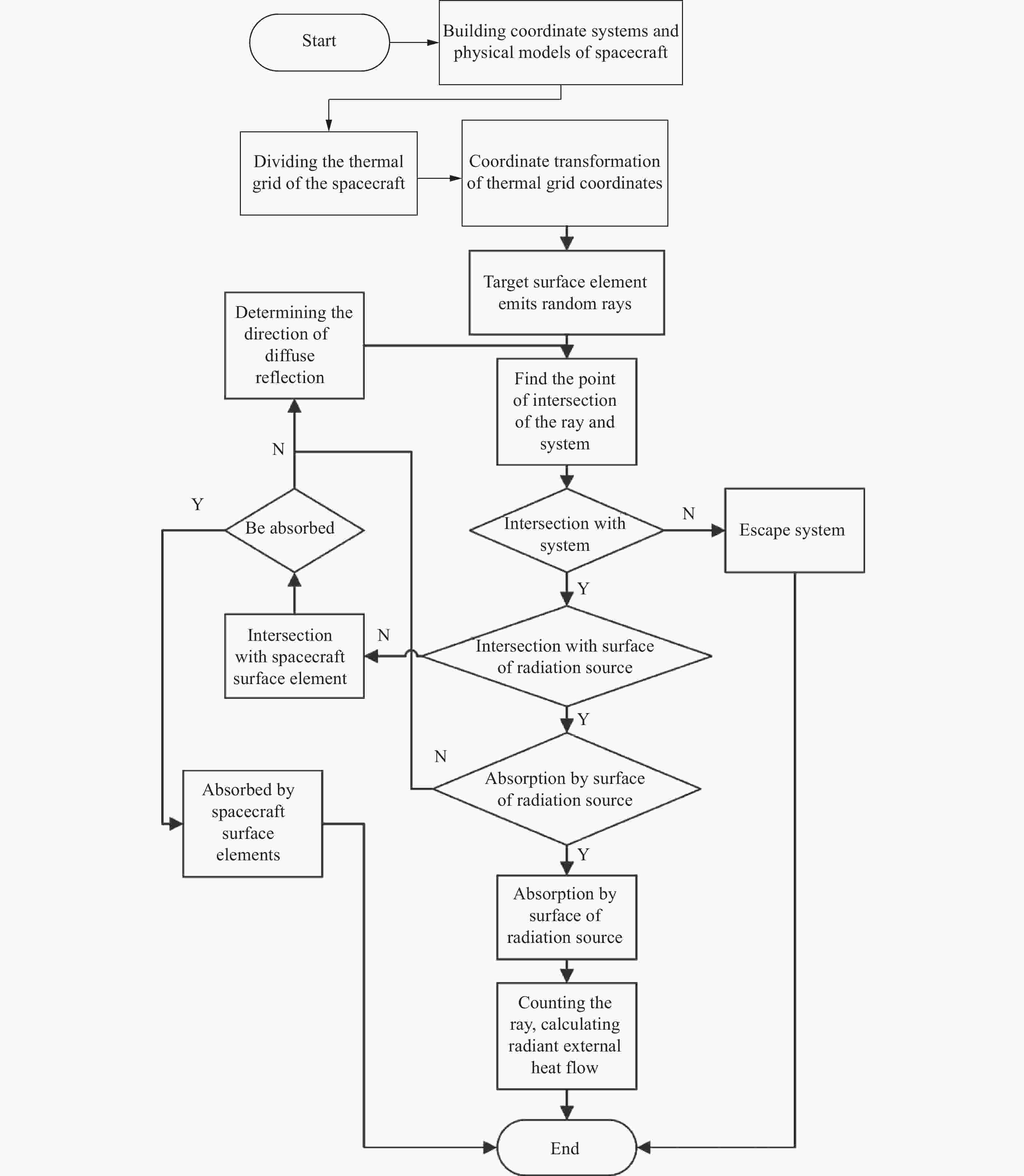
图 1 单束光线的反向蒙特卡洛模拟
Figure 1. Inverse Monte Carlo simulation of a single ray
具体步骤如下:
1)建立本体坐标系、轨道坐标系、地心惯性坐标系等参照坐标系,给出轨道参数;
2)建立航天器结构热物理模型,划分热分析面元网格,确定各热分析面元表面方程及辐射特性;
3)航天器某一目标面元表面发射随机光线;
4)求解光线与系统(航天器与辐射源)面元的交点,并分析此光线被吸收还是反射,若被反射则继续跟踪;
5)如果光线被辐射源表面吸收,则按反向过程统计光线对目标面元表面的外热流;
6)如果光线被航天器面元吸收或者逸出,则不再跟踪。
-
在外热流模拟计算中,需要对航天器表面进行离散化处理。对于复杂的三维表面,通常采用有限数量的三角形面元进行离散表示。热网格面元划分标准为在每个三角形面元范围内,物理量如温度和发射率等数值基本均匀。每个三角形面元由三个顶点和面元外法向量表示。
对于三角形面元,根据公式(7)确定光线的随机发射点[31]为:
$$ {\boldsymbol{r}} = {{\boldsymbol{r}}_{\text{0}}}(1 - {{s}} - {{t}}) + {{\boldsymbol{r}}_{\text{1}}}{{s}} + {{\boldsymbol{r}}_{\text{2}}}{{t}} $$ (7) 式中:r为光线的随机发射点;r0、r1、r2为三角形三个顶点的坐标;s和t的值可以通过公式(8)求解得到:
$$ s = {R_{2r}}\sqrt {{R_{1r}}} ,t = \sqrt {{R_{1r}}} (1 - {R_{2r}}) $$ (8) 式中:R1r、R2r为区间[0,1]内均匀分布的随机数。
利用切球法[18]对漫发射面元上光线随机发射方向进行模拟,其天顶角θ和周向角ψ的值可以通过公式(9)求解得到:
$$ \theta {\text{ = }}\arccos (1 - 2{R_\theta }),\psi = 2\pi {R_\psi } $$ (9) 式中:Rθ、Rψ为区间[0,1]内均匀分布的随机数。
-
通过光线发射点和发射方向的概率模拟,得出目标面元所发随机光线的方程。联立求解系统表面与目标面元随机光线方程组,以判断光线是否与之有交点。若方程存在多个解,说明光线与系统内多个面元相交,需取光线传播距离最短情况下的交点。
如果光线和整个系统都没有交点,则视光线逸出并进入太空。若光线和系统表面有交点,则需要判断光线是否被吸收或反射。判断方式如下,产生区间[0,1]内均匀分布的随机数Rα,若满足公式(10),则光线被吸收,该束光线追踪过程结束。若满足公式(11),则光线被反射,需从交点发射一束随机光线作为漫反射的光线继续追踪,其反射方向模拟与发射方向模拟方法相同。
$$ {R_\alpha } \leqslant \alpha $$ (10) $$ \alpha < {R_\alpha } \leqslant 1 $$ (11) 式中:α为交点所在面元的光谱吸收率。
最终为计算目标面元地球红外和反照辐射的外热流,只需统计被辐射源(地球)表面吸收的随机光线数目即可。
-
在计算地球红外辐射外热流时,将地球视为发射率为1的黑体。基于地球红外辐射能量守恒关系及RMC法基本原理,从航天器目标面元发射光线,并跟踪从面元i发出的Nei束光线,若有Nai束到达地球表面并被吸收,则面元i吸收的地球红外辐射外热流密度为:
$$ q_i^{{r}} = \frac{1}{{{N_{{\text{ei}}}}}}\left({N_{{\text{ai}}}} \cdot \frac{{1 - \rho }}{4} \cdot S \cdot {\varepsilon _{{i}}}^{{r}} \cdot \frac{1}{{\varepsilon _{{e}}^{{r}}}}\right) $$ (12) 式中:ρ为地球的平均太阳反照率,其值为0.35;S为太阳常数,其值为1353 W/m2;${\varepsilon _{{i}}}^{{r}}$为面元i涂层的红外发射率;${\varepsilon _{{e}}}^{{r}}$为地球红外发射率,其值为1。
-
基于地球反照辐射的能量守恒关系及RMC法的基本原理,从航天器目标面元发射光线,并跟踪从面元i发出的Nei束光线,若有Nai束到达地球表面并被吸收,并且其与地球交点外法线向量和太阳光线方向向量的夹角θse大于90°,则面元i吸收的地球反照辐射外热流密度为:
$$ q_i^{{\text{er}}} = \frac{1}{{{N_{{\text{ei}}}}}}\left(\sum\limits_{j = 1}^{{N_{{\text{ai}}}}} \rho \cdot S \cdot {\alpha _i}^{{s}} \cdot \left| {\cos {\theta _j}^{{\text{se}}}} \right| \cdot \frac{1}{{\alpha _e^s}}\right) $$ (13) 式中:αis为面元i涂层的太阳吸收率;αes为地球的平均太阳吸收率,其值为0.65。
-
在上述光线追踪过程中,统计地球红外和反照辐射外热流与目标面元光线发射点的位置和发射方向、相交后是否反射、反射方向等变量有关,这些变量由仿真过程产生的随机数决定。其中随机数R1r和R2r决定目标面元光线发射点的位置,随机数Rθ和Rψ决定目标面元光线发射方向和光线相交后的反射方向,随机数Rα决定光线相交后是否反射。
d为目标面元地球红外和反照辐射外热流积分所需的变量维度。在这里,变量维度d对应于初始化和跟踪光线的不同随机变量的数量。光线iray为目标面元所发光线中反射次数最多的光线,则外热流积分变量维度d的求解公式如下:
$$ d = \left\{ {\begin{array}{*{20}{l}} 4 &\begin{array}{l} {\rm{If\; the \; ray, }}\;{i_{{\rm{ray}}}},\;{\rm{ does \;not \;intersect }}\\ {\rm{with\; the\; system's \;surface}}\\ {\rm{and \;proceeds\; to\; escape \;directly}}.\\ \end{array}\\ {3{N_1} + 2}&\begin{array}{l} {\rm{If \;the\; ray, }}\;{i_{{\rm{ray}}}},\;{\rm{ intersects\; with }}\\ {\rm{the\; system's\; surface }}\;{N_1}\;{\rm{ times, }}\\ {\rm{thereafter\; being \;absorbed \;by }}\\ {\rm{the \;surface}}.\\ \end{array}\\ {3{N_1} + 4}&\begin{array}{l} {\rm{If\; the\; ray,}}\;{i_{{\rm{ray}}},}\;{\rm{ intersects\; with }}\\ {\rm{the \;system's \;surface\; }}\;{N_1}\;{\rm{ times, }}\\ {\rm{subsequently \;being\; reflected }}\\ {\rm{and \;escaping \;the \;system}}{\rm{.}} \end{array} \end{array}} \right. $$ (14) 式中:N1>0。
在外热流积分的计算中,并非所有维度都拥有同等的重要性。目标面元发射的所有光线,都需要产生初始光线的发射点和发射方向,需要利用到随机数R1r、R2r、Rθ和Rψ,也就是积分前四维的重要性大于其他积分维度。
-
为了改善传统MC样本的丛聚现象,文中基于QMC对传统地球红外和反照辐射外热流求解方法进行改进。
当目标面元发射光线数目一定时,不同于传统MC样本构造,QMC样本构造需要预先知道问题的变量维度。若选择构造样本的变量维度过大,则会对目标面元发射的每束光线构造相同维度的样本。但由于存在目标面元发出的光线未被反射的情况,将导致产生未被用到的样本,从而浪费内存资源。并且QMC在变量维度较高和一定样本量下并不优于MC[26]。
综合考虑地球红外和反照辐射外热流积分各维度的重要性以及QMC样本的构造需求,文中将QMC和MC混合到一起,对于外热流积分的前四个维度,采用QMC产生的样本代替MC产生的样本,而外热流积分其他维度仍采用MC产生的样本。由于只对外热流积分前四维度进行改进,所以文中的QMC采用的拟随机数序列为Halton序列。
-
MC误差的阶为O(N −1/2),误差与积分维度无关。LHS所得到的最差结果相当于少采用一个样本点的MC[32],其误差的阶最坏情况为O(N −1/2)。QMC误差的阶最好情况为O(N −1),最坏情况为O((lnvN)N −1) [33]。
对于外热流积分来说,N代表目标面元发射的光线数量,v为该方法产生样本的积分维度。由于传统方法和混合-QMC对反射光线所需样本的处理都为MC,只有外热流积分前四维度的样本为不同方法,所以v=4。在光线数量一定时,各方法误差的阶越小,该方法越好。
LHS误差的阶最坏情况与MC误差的阶相等,说明LHS优于MC。当v=4且在一定光线数量N下,MC误差的阶落在QMC误差的阶最好情况和最坏情况之间。为具体比较这两种方法处理外热流问题误差的阶,需获得QMC处理外热流问题误差的阶。文中基于混合-QMC计算外热流问题的准确度和收敛速度,来获得该方法处理外热流问题误差的阶。
-
图2为文中研究的航天器热分析模型,该模型由星本体(红色)、太阳帆板(浅蓝色)、天线(紫色)和桁架(深蓝色)组成。此处的航天器面元编号与下述实验分析所使用的面元编号一致。轨道空间外热流只作用于该航天器的外表面上,因此文中不涉及其内部结构。航天器轨道和姿态参数见表1,结构涂层表面辐射特性参数见表2。

图 2 航天器热分析模型及分析面元编号图
Figure 2. Diagram of spacecraft thermal analysis model and analysis surface elements number
表 1 轨道及姿态参数
Table 1. Orbit and attitude parameters
Parameters Numerical value Semimajor axis/km 6878 Eccentricity 0 Orbit inclination/(°) 0 Attitude Z-axis to ground orientation 表 2 结构涂层表面辐射特性参数
Table 2. Radiation characteristic parameters of structural coating surface
Spacecraft structure Surface solar absorptivity Surface infrared emissivity Satellite body 0.46 0.63 Antennae 0.65 0.72 Solar panel 0.41 0.59 Truss 0.56 0.68 根据图2可知,该航天器被离散成许多面元,每个航天器表面由正面面元和反面面元组成。在假设正反面温差较小的情况下,采用相同编号来标识正面面元和反面面元,即它们是同一面元。
-
航天器、地球和太阳的相对位置关系如图3所示,可以看出,当前时刻该航天器处于光照区。首先对图3位置处的航天器所吸收的地球红外和反照辐射外热流密度进行仿真编程和代码校验,该航天器共由40个面元组成。

图 3 航天器位置图
Figure 3. Spacecraft location picture
Thermal Desktop(TD)软件为当前航天器热分析的主流软件之一,其中计算地球辐射外热流的方法为MC。为了验证所编程序的准确性,以TD软件计算结果为基准,与自编MC计算外热流密度程序结果进行比较。在TD软件和自编程序中,每个面元均发射2×10⁶束光线,来计算地球辐射外热流。通过对比软件和程序仿真结果,获得40个面元所吸收地球红外和反照辐射外热流密度相对误差绝对值的平均值,其值也被称为平均相对误差。
对于航天器所吸收的地球反照辐射外热流密度,所有面元的平均相对误差为0.52%。而对于航天器所吸收的地球红外辐射外热流密度,所有面元的平均相对误差为0.61%。
综上,认为编写航天器所吸收的地球红外和反照辐射外热流密度程序准确无误。
-
从航天器帆板、星本体、天线以及桁架结构中各选取一个面元作为研究对象,分析传统方法和改进方法计算面元所吸收的地球红外和反照辐射外热流密度的准确度。
各方法的准确性由平均解的实际误差(来自精确解)或被评估变量在多次统计迭代上的标准差(即其统计误差)决定。各方法解的准确性是通过使用较少的样本进行大量模拟来估计,而不是使用相同的样本总数进行单一模拟。
基于传统方法和改进方法,面元i发射N束光线,计算所吸收的地球红外和反照辐射外热流密度。重复执行上述过程M次,得到M个对应结果,对其结果进行分析,即可得出各方法的准确度,准确度求解过程如下。
平均解的实际误差为局部均方根(RMS)相对误差,求解公式如下:
$$ {\varepsilon _i} = {\left[ {\frac{1}{M}\sum\limits_{m = 1}^M {{{\left(\frac{{P_i^m}}{{P_i^o}} - 1\right)}^2}} } \right]^{1/2}} $$ (15) 式中:P为解决方案的目标变量,在文中目标变量为面元i所吸收的地球红外和反照辐射的外热流密度;M为统计运行次数;$ P_{i}^{m} $为面元i 第m次蒙特卡洛模拟采样值;$ P_{i} $为面元i基准解;εi为面元i目标变量的局部均方根相对误差。
传统的概率统计方法用于计算被评估变量在多次统计迭代上的标准差。
不同于MC和LHS,QMC产生的样本不具有随机性。若采用该方法重复生成样本,则将始终产生相同的样本。为了估计标准差和局部均方根的相对误差,需要确保在每次QMC模拟中使用的实际样本序列都不同。根据文献[34],可以通过以下方法来满足该要求。
首先产生具有M×N个样本的四维拟随机数序列,表示为:
$$ \begin{split} {S_4} =& [(S_1^1,S_1^2,S_1^3,S_1^4),(S_2^1,S_2^2,S_2^3,S_2^4), \cdots , \\ & (S_{MN}^1,S_{MN}^2,S_{MN}^3,S_{MN}^4)] \\ \end{split} $$ (16) 然后使用从该子集生成的光线来运行第m个具有N束光线的QMC实例:
$$ \begin{split} & [(S_{(m - 1)N + 1}^1,S_{(m - 1)N + 1}^2,S_{(m - 1)N + 1}^3,S_{(m - 1)N + 1}^4), \cdots , \\ &(S_{mN}^1,S_{mN}^2,S_{mN}^3,S_{mN}^4)], \\ & m = [1,2,\cdots ,M] \\ \end{split} $$ (17) 根据定义,QMC样本的任何子集也是QMC样本,因此该第m个子集充当不同的QMC样本。
综上,在重复计算面元i所吸收的地球红外和反照辐射外热流密度M次的过程中,QMC产生的样本按照上述过程进行。最后,应使用传统的概率统计方法计算得出结果的标准差。
-
实验分析面元编号及其对应的航天器部件,如表3所示,可以通过图2确定实验分析面元的具体位置。
表 3 航天器实验分析面元编号及所属部件
Table 3. Spacecraft experiment analysis surface elements numbers and their components
Number of
surface elementsSpacecraft components belonging to
surface elements1 Satellite body 15 Solar panel 21 Antennae 40 Truss 为求解各种方法计算外热流的准确度,需要重复求解目标单元外热流M次。文中综合考虑计算量和各方法外热流准确度的精确程度,设计了外环循环实验,以获得合理的M值。
为得到各种方法计算外热流的收敛速度和误差的阶,需从面元发射出多种工况光线数。文中通过改变光线数N来获得各种方法收敛速度和误差的阶,并设计了内环循环实验来实现这一目的。
综上,通过图4来说明文中所设计的实验。在其他条件不变的情况下,通过改变面元发射光线数N来探究各种方法计算外热流的收敛速度,从而设计了内环循环实验。同样在其他条件不变的情况下,通过改变外环循环实验次数M来获得合理的M值,进而设计了外环循环实验。
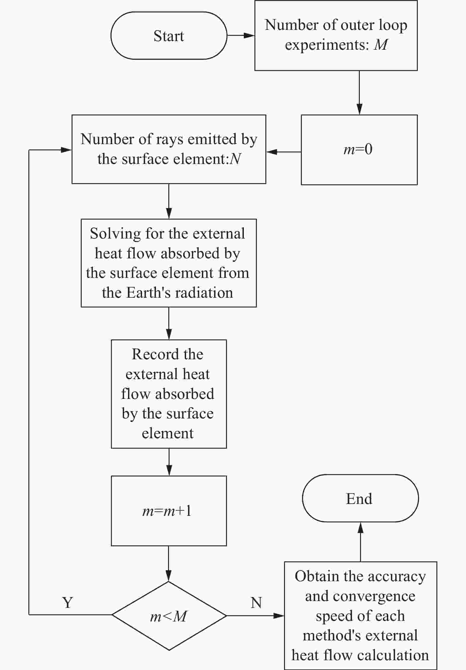
图 4 各方法外热流计算准确度和收敛速度求解流程图
Figure 4. Calculation accuracy of external heat flow and solution flow chart of convergence speed of each method
-
由于外热流计算方法准确度的求解需要多次运行实验工况M次,文中选取M值为1000。为分析验证M取值是否合理,设计了如下实验。
针对内环循环实验工况五,基于传统方法和改进方法分别对其运行M次,实验次数M的选取见表4,通过求解各实验对应的局部均方根相对误差和标准差,以判断M取值的合理性。
表 4 外环循环实验设计-各面元实验工况五运行次数
Table 4. Design of the outer loop cycle experiment-running times of the experimental conditions five of each surface elements
Number of outer loop
cycle experimentRunning times of
experimental conditions fiveExperiment 1 100 Experiment 2 200 Experiment 3 300 Experiment 4 400 Experiment 5 500 Experiment 6 600 Experiment 7 700 Experiment 8 800 Experiment 9 900 Experiment 10 1000 Experiment 11 2 000 Experiment 12 3000 Experiment 13 4000 Experiment 14 5000 Experiment 15 6000 Experiment 16 7000 Experiment 17 8000 Experiment 18 9000 Experiment 19 10000 -
为了比较传统方法和改进方法计算外热流的准确度和收敛性能,需从面元发出不同的光线数,计算不同种工况下面元所吸收的外热流密度。文中根据所发光线数设计了七种实验工况,并为评估各种方法的准确性增设了一个基准工况,用于求解局部均方根的相对误差。各面元求解外热流所发光线数对应的实验工况如表5所示。
表 5 内环循环实验设计-各面元实验工况所发光线数
Table 5. Experimental design of the inner loop-number of rays emitted by each surface elements experimental condition
Experimental conditions
in the inner loopSurface
element 1Surface element
15, 21, 40Experimental condition one 1000 2 000 Experimental condition two 5000 10000 Experimental condition three 10000 20000 Experimental condition four 50000 100000 Experimental condition five 100000 200000 Experimental condition six 500000 1000000 Experimental condition seven 1000000 2000000 由表5可知,面元1所发光线数为其他面元发射光线数的一半。这是由于面元1在部件星本体上,星本体内部不受外热流作用,其外热流为0,面元1仅单面受外热流影响,其他面元正反面均受到外热流的影响。
对于基准工况,基于MC计算面元所吸收的地球红外和反照辐射外热流密度,面元1所发光线数为1×10⁹,面元15、21、40所发光线数为2×10⁹。计算所得数值作为求解局部均方根相对误差公式中的基准解。
最后为获得外热流计算方法的准确度,对工况一~工况七进行了1000次运行。将所得结果代入公式(15)和标准差求解公式中,得到各工况对应的局部均方根相对误差和标准差。
-
图5和图6为航天器面元各方法外环循环实验外热流的准确度。从图中可以看出,在实验工况五下,不同面元使用各种外热流求解方法100~10000次运行后,地球反照和红外辐射外热流的标准差和RMS相对误差在运行次数达到1000之后的变化趋于稳定。以上结果证明了文中循环实验M取1000次的合理性。

图 5 航天器面元各方法外环循环实验地球反照外热流的准确度
Figure 5. Accuracy of external heat flow of Earth albedo in the outer loop loop experiment of each method of spacecraft surface elements
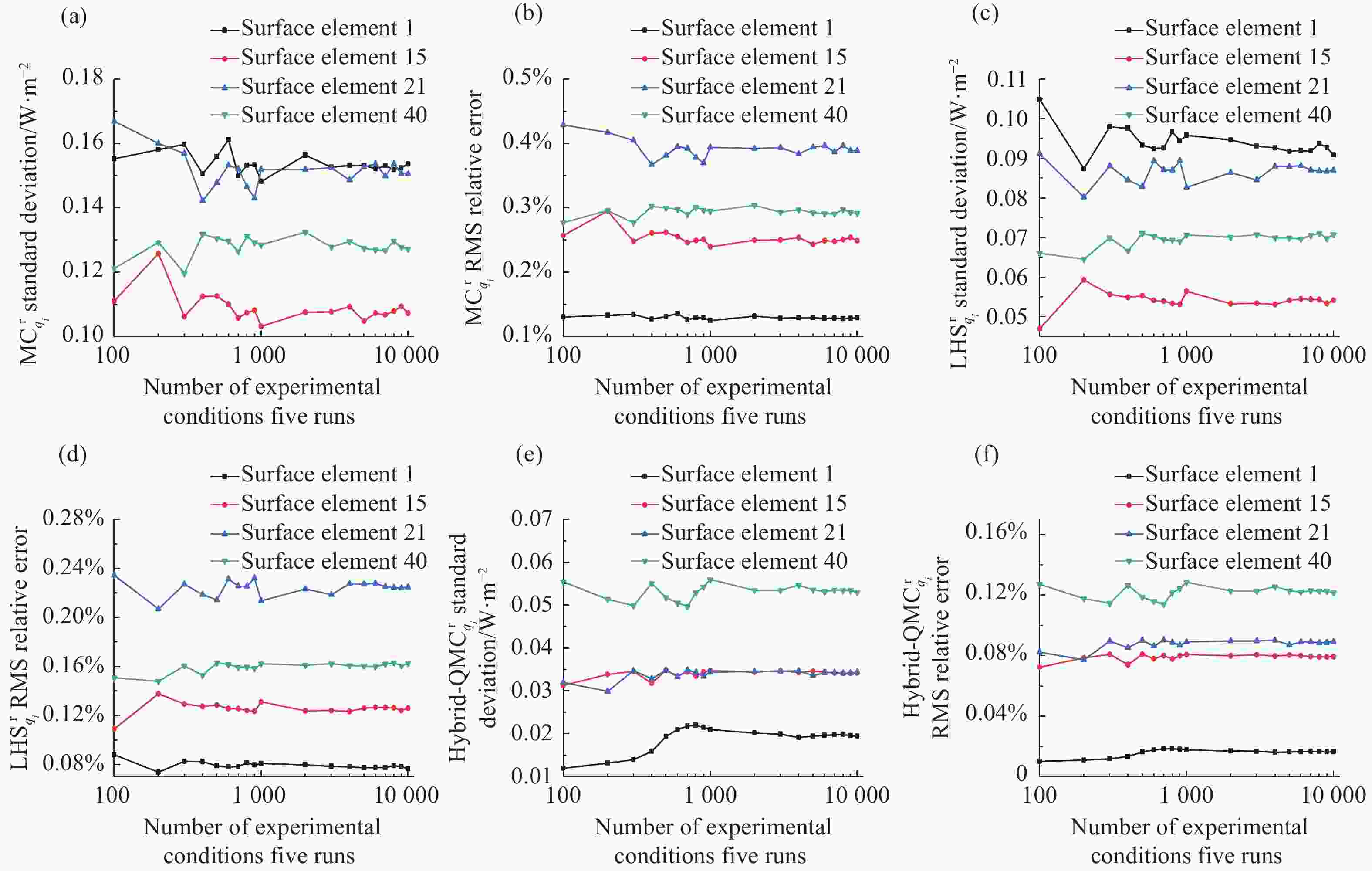
图 6 航天器面元各方法外环循环实验地球红外外热流的准确度
Figure 6. Accuracy of external heat flow of Earth infrared in the outer loop loop experiment of each method of spacecraft surface elements
图7和图8为面元各方法地球辐射外热流求解的准确度,根据图7和图8,可以得出以下结果:

图 7 航天器面元各方法内环循环实验地球反照辐射外热流的准确度
Figure 7. Accuracy of the external heat flow of the Earth albedo radiation in the inner loop experiment of each method of the spacecraft surface elements
1)应用以上三种方法求解外热流,各面元地球反照和红外辐射外热流的标准偏差和实际误差都随面元所发光线数量的增加而减少。
2)相同面元发射相同光线数量,各算法地球反照和红外辐射外热流标准偏差比较:对所有面元来说,混合-QMC标准偏差<LHS标准偏差<MC标准偏差。
3)相同面元发射相同光线数量,各算法地球反照和红外辐射RMS相对误差比较:对所有面元来说,混合-QMC RMS相对误差<LHS RMS相对误差<MC RMS相对误差。
综上,根据所得结果可知,计算地球红外和反照辐射外热流三种方法的准确度,混合-QMC最优,LHS次之,MC最差。
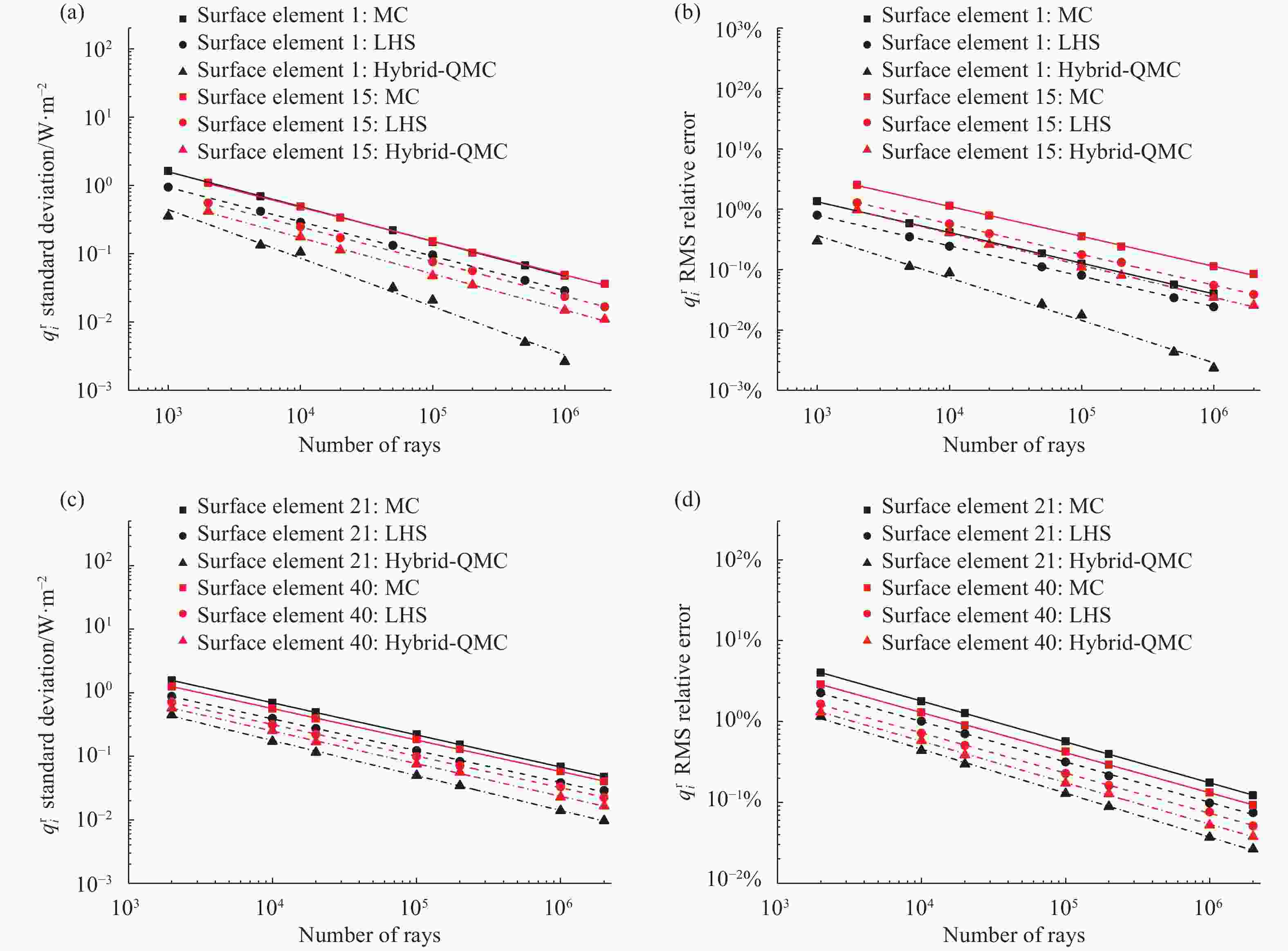
图 8 航天器面元各方法内环循环实验地球红外辐射外热流的准确度
Figure 8. Accuracy of the external heat flow of the Earth infrared radiation in the inner loop experiment of each method of the spacecraft surface elements
-
图7和图8中各种算法对应散点所拟合直线的斜率为该种方法对应面元地球反照和红外辐射外热流的标准差和RMS相对误差的收敛速度[35],并且该收敛速度等于方法处理外热流问题误差的阶N上面的指数值。例如,MC误差的阶为O(N −1/2),则理论上MC对应的收敛速率应为−0.5。直线斜率绝对值越大,该直线所对应的收敛速度越快,各方法收敛速度详见表6~表9。
表 6 三种方法各面元地球反照辐射外热流标准差的收敛速度
Table 6. Convergence speed of the standard deviation of the external heat flow of the Earth albedo radiation in each surface elements of the three methods
Standard deviation
convergence speedMC LHS Hybrid-QMC Surface element 1 −0.4947 −0.5015 −0.7132 Surface element 15 −0.4981 −0.4967 −0.5221 Surface element 21 −0.5003 −0.4998 −0.5335 Surface element 40 −0.5004 −0.5047 −0.5104 表 7 三种方法各面元地球反照辐射外热流RMS相对误差的收敛速度
Table 7. Convergence speed of the RMS relative error of the external heat flow of the Earth albedo radiation in each surface elements of the three methods
RMS relative error
convergence speedMC LHS Hybrid-QMC Surface element 1 −0.4945 −0.5013 −0.7110 Surface element 15 −0.4979 −0.4967 −0.5220 Surface element 21 −0.5006 −0.4999 −0.5333 Surface element 40 −0.5004 −0.5045 −0.5099 表 8 三种方法各面元地球红外辐射外热流标准差的收敛速度
Table 8. Convergence speed of the standard deviation of the external heat flow of the Earth infrared radiation in each surface elements of the three methods
Standard deviation
convergence speedMC LHS Hybrid-QMC Surface element 1 −0.5089 −0.5035 −0.7093 Surface element 15 −0.4963 −0.5064 −0.5294 Surface element 21 −0.5051 −0.5000 −0.5501 Surface element 40 −0.4956 −0.4968 −0.5137 表 9 三种方法各面元地球红外辐射外热流RMS相对误差的收敛速度
Table 9. Convergence speed of the RMS relative error of the external heat flow of the Earth infrared radiation in each surface elements of the three methods
RMS relative error
convergence speedMC LHS Hybrid-QMC Surface element 1 −0.5089 −0.5035 −0.7032 Surface element 15 −0.4963 −0.5063 −0.5293 Surface element 21 −0.5049 −0.4992 −0.5431 Surface element 40 −0.4957 −0.4966 −0.5133 根据表6~表9可知,对于所有面元,混合-QMC所求地球反照和红外辐射外热流标准差和RMS相对误差的收敛速度均优于其他两种方法。值得注意的是,面元1使用混合-QMC求解地球辐射外热流,其收敛速度提升的效果最好。原因在于,在光线追踪的过程中,面元1发出的光线未发生反射,没有经过航天器表面其他面元,而其他三个面元发出的光线则会经过航天器表面其他面元进行反射。表10和表11为传统方法内环循环实验工况七,面元发射光线的最大反射次数。在光线击中航天器表面其他面元并发生反射的过程中,外热流积分变量的维度会增加,这些新增的积分变量仍使用MC来采样。由于面元1的外热流求解过程中没有增加上述积分变量的维度,因此其收敛速度提升的效果最佳。
表 10 内环循环实验工况七地球红外辐射外热流求解光线追踪过程中面元所发光线的最大反射次数
Table 10. Maximum reflection number of ray emitted by surface elements during ray tracing for the inner loop experimental condition seven Earth infrared radiation external heat flow solution
Number of surface elements Maximum number of ray reflections 1 0 15 7 21 6 40 6 表 11 内环循环实验工况七地球反照辐射外热流求解光线追踪过程中面元所发光线的最大反射次数
Table 11. Maximum reflection number of light emitted by a surface elements during ray tracing for the inner loop experimental condition seven Earth albedo radiation external heat flow solution
Number of surface elements Maximum number of ray reflections 1 0 15 7 21 9 40 10 综上,采用混合-QMC方法求解地球反照和红外辐射外热流时,其收敛速度优于其他两种方法。在对各个面元进行光线追踪求解地球辐射外热流的过程中,不存在反射光线的面元能够获得更好的收敛速度。对这些面元而言,混合-QMC方法的外热流准确性收敛速度提升的效果最为显著。
-
1)文中分析了地球辐射外热流中各个积分变量维度的重要性,结果表明,前四个积分维度对地球反照和红外辐射外热流积分的贡献最大。
2)文中基于QMC改进传统蒙特卡洛外热流计算方法,将QMC和MC结合到一起求解地球辐射外热流。根据误差阶理论,无法比较QMC和MC方法计算地球反照和红外辐射外热流的优劣。因此,以某航天器为例进行计算,结果显示,混合-QMC方法在处理航天器不同面元的外热流时,具有最高的准确性和收敛速度。
3)在面元地球辐射外热流求解过程中,统计面元所发射的光线,若这些光线中不存在光线的反射行为,混合-QMC对该面元地球辐射外热流准确度收敛速度提升的效果最好。
综上,基于混合-QMC方法计算航天器地球红外和反照辐射外热流比其他两种方法更优。当面元发射的光线不存在反射行为时,混合-QMC的优势更加突出。该方法可为提高航天器外热流计算速度和精度提供一定的参考。
Assessment of hybrid-quasi-Monte Carlo method efficiency in Earth radiative external heat flow calculation
-
摘要: 空间外热流仿真计算是航天器热控设计以及地面试验验证的关键技术之一。传统蒙特卡洛法(MC)抽样的随机性问题导致其计算地球红外和反照辐射外热流的收敛速度慢。为解决这一问题,文中首先分析比较外热流积分各个随机变量维度对积分的贡献程度,发现前四维随机变量对积分贡献程度最高。之后在外热流积分的前四维度中,将拟蒙特卡洛法(QMC)代替传统MC,对所求目标面元光线发射点和方向进行采样,其他积分维度仍采用MC,该方法将MC和QMC混合到一起计算外热流。最后以某航天器为算例,通过大数据光线追踪实验得出外热流准确度和收敛速度。研究结果表明,混合-QMC计算地球红外和反照辐射外热流的准确度始终优于传统方法。进一步的分析表明,该方法在地球辐射外热流准确度上的收敛速率,优于传统方法所呈现的收敛速度值(即-0.5)。此外,在面元地球辐射外热流求解的光线追踪过程中,若面元所发光线不存在反射的情况,混合-QMC方法能够更准确快速地求解其外热流。将混合-QMC应用到地球辐射外热流计算中,可以在一定程度上提高计算效率。Abstract:
Objective The computational simulation of external heat flux in space is a crucial aspect of spacecraft thermal management design and ground test validation. Monte Carlo (MC) techniques are currently the prevailing approach for addressing spacecraft external heat flux calculations. Nevertheless, the inherent shortcoming of MC methods is their comparatively slow rate of convergence. To achieve a statistical solution for the external heat flux approximating the precise solution, a considerable number of rays must be emitted, resulting in substantial computational overhead. Consequently, the exploration of efficient algorithms for solving external heat flux is of paramount importance. To this end, a comprehensive examination of Earth radiative external heat flux is conducted, leading to the development of an innovative computational algorithm. The findings of this study will offer valuable theoretical insights for enhancing the calculation efficiency of Earth infrared and albedo radiation external heat flux, and serve as a reference for research on the localization of spacecraft external heat flux computation software. Methods Firstly, an analysis and comparison of the contribution of each random variable dimension within the Earth radiative external heat flux integral are conducted, revealing that the foremost four dimensions of random variables yield the most significant contributions to the integral. Subsequently, Quasi-Monte Carlo (QMC) techniques are employed in lieu of traditional MC methods for the first four dimensions of the external heat flux integral to sample the ray emission point and direction for the target surface element in question, while MC is utilized for the remaining integration dimensions. This novel algorithm combines both MC and QMC approaches to compute the external heat flux. Lastly, a spacecraft serves as a computational example to ascertain the accuracy and convergence rate of the external heat flux through a large-scale ray tracing experiment. Results and Discussions The comparative accuracy of the three methods employed to calculate Earth infrared and albedo external heat flux reveals the superior performance of hybrid-QMC, followed by Latin Hypercube Sampling (LHS), and lastly, the least accurate being MC (Fig.7-8). When utilizing the hybrid-QMC approach to solve Earth albedo and infrared radiative external heat flux, the convergence rate surpasses that of the other two methods. In ray tracing individual surface elements to solve the Earth radiative external heat flow, the surface elements without reflected rays can obtain a better convergence speed. For these surface elements, the hybrid-QMC method has the most significant improvement in the convergence speed of the external heat flow accuracy (Tab.6-9). Conclusions The importance of each integration variable dimension in the Earth radiative external heat flow is analyzed, and the results show that the first four integration dimensions contribute the most to the integration of the Earth albedo and infrared radiative external heat flow. A spacecraft is used as an example for calculation, and the results show that the hybrid-QMC method has the highest accuracy and convergence speed when dealing with the external heat flow of different surface elements of the spacecraft. The advantage of hybrid-QMC is more prominent when there is no reflection behavior of the ray emitted by the surface element. This method can provide some reference to improve the speed and accuracy of the spacecraft external heat flow calculation. -
图 2 航天器热分析模型及分析面元编号图
Figure 2. Diagram of spacecraft thermal analysis model and analysis surface elements number
图 4 各方法外热流计算准确度和收敛速度求解流程图
Figure 4. Calculation accuracy of external heat flow and solution flow chart of convergence speed of each method
图 5 航天器面元各方法外环循环实验地球反照外热流的准确度
Figure 5. Accuracy of external heat flow of Earth albedo in the outer loop loop experiment of each method of spacecraft surface elements
图 6 航天器面元各方法外环循环实验地球红外外热流的准确度
Figure 6. Accuracy of external heat flow of Earth infrared in the outer loop loop experiment of each method of spacecraft surface elements
图 7 航天器面元各方法内环循环实验地球反照辐射外热流的准确度
Figure 7. Accuracy of the external heat flow of the Earth albedo radiation in the inner loop experiment of each method of the spacecraft surface elements
图 8 航天器面元各方法内环循环实验地球红外辐射外热流的准确度
Figure 8. Accuracy of the external heat flow of the Earth infrared radiation in the inner loop experiment of each method of the spacecraft surface elements
表 1 轨道及姿态参数
Table 1. Orbit and attitude parameters
Parameters Numerical value Semimajor axis/km 6878 Eccentricity 0 Orbit inclination/(°) 0 Attitude Z-axis to ground orientation  下载: 导出CSV
表 2 结构涂层表面辐射特性参数
Table 2. Radiation characteristic parameters of structural coating surface
Spacecraft structure Surface solar absorptivity Surface infrared emissivity Satellite body 0.46 0.63 Antennae 0.65 0.72 Solar panel 0.41 0.59 Truss 0.56 0.68
下载: 导出CSV
表 3 航天器实验分析面元编号及所属部件
Table 3. Spacecraft experiment analysis surface elements numbers and their components
Number of
surface elementsSpacecraft components belonging to
surface elements1 Satellite body 15 Solar panel 21 Antennae 40 Truss
下载: 导出CSV
表 4 外环循环实验设计-各面元实验工况五运行次数
Table 4. Design of the outer loop cycle experiment-running times of the experimental conditions five of each surface elements
Number of outer loop
cycle experimentRunning times of
experimental conditions fiveExperiment 1 100 Experiment 2 200 Experiment 3 300 Experiment 4 400 Experiment 5 500 Experiment 6 600 Experiment 7 700 Experiment 8 800 Experiment 9 900 Experiment 10 1000 Experiment 11 2 000 Experiment 12 3000 Experiment 13 4000 Experiment 14 5000 Experiment 15 6000 Experiment 16 7000 Experiment 17 8000 Experiment 18 9000 Experiment 19 10000
下载: 导出CSV
表 5 内环循环实验设计-各面元实验工况所发光线数
Table 5. Experimental design of the inner loop-number of rays emitted by each surface elements experimental condition
Experimental conditions
in the inner loopSurface
element 1Surface element
15, 21, 40Experimental condition one 1000 2 000 Experimental condition two 5000 10000 Experimental condition three 10000 20000 Experimental condition four 50000 100000 Experimental condition five 100000 200000 Experimental condition six 500000 1000000 Experimental condition seven 1000000 2000000
下载: 导出CSV
表 6 三种方法各面元地球反照辐射外热流标准差的收敛速度
Table 6. Convergence speed of the standard deviation of the external heat flow of the Earth albedo radiation in each surface elements of the three methods
Standard deviation
convergence speedMC LHS Hybrid-QMC Surface element 1 −0.4947 −0.5015 −0.7132 Surface element 15 −0.4981 −0.4967 −0.5221 Surface element 21 −0.5003 −0.4998 −0.5335 Surface element 40 −0.5004 −0.5047 −0.5104
下载: 导出CSV
表 7 三种方法各面元地球反照辐射外热流RMS相对误差的收敛速度
Table 7. Convergence speed of the RMS relative error of the external heat flow of the Earth albedo radiation in each surface elements of the three methods
RMS relative error
convergence speedMC LHS Hybrid-QMC Surface element 1 −0.4945 −0.5013 −0.7110 Surface element 15 −0.4979 −0.4967 −0.5220 Surface element 21 −0.5006 −0.4999 −0.5333 Surface element 40 −0.5004 −0.5045 −0.5099
下载: 导出CSV
表 8 三种方法各面元地球红外辐射外热流标准差的收敛速度
Table 8. Convergence speed of the standard deviation of the external heat flow of the Earth infrared radiation in each surface elements of the three methods
Standard deviation
convergence speedMC LHS Hybrid-QMC Surface element 1 −0.5089 −0.5035 −0.7093 Surface element 15 −0.4963 −0.5064 −0.5294 Surface element 21 −0.5051 −0.5000 −0.5501 Surface element 40 −0.4956 −0.4968 −0.5137
下载: 导出CSV
表 9 三种方法各面元地球红外辐射外热流RMS相对误差的收敛速度
Table 9. Convergence speed of the RMS relative error of the external heat flow of the Earth infrared radiation in each surface elements of the three methods
RMS relative error
convergence speedMC LHS Hybrid-QMC Surface element 1 −0.5089 −0.5035 −0.7032 Surface element 15 −0.4963 −0.5063 −0.5293 Surface element 21 −0.5049 −0.4992 −0.5431 Surface element 40 −0.4957 −0.4966 −0.5133
下载: 导出CSV
表 10 内环循环实验工况七地球红外辐射外热流求解光线追踪过程中面元所发光线的最大反射次数
Table 10. Maximum reflection number of ray emitted by surface elements during ray tracing for the inner loop experimental condition seven Earth infrared radiation external heat flow solution
Number of surface elements Maximum number of ray reflections 1 0 15 7 21 6 40 6
下载: 导出CSV
表 11 内环循环实验工况七地球反照辐射外热流求解光线追踪过程中面元所发光线的最大反射次数
Table 11. Maximum reflection number of light emitted by a surface elements during ray tracing for the inner loop experimental condition seven Earth albedo radiation external heat flow solution
Number of surface elements Maximum number of ray reflections 1 0 15 7 21 9 40 10
下载: 导出CSV
-
[1] Wang Shuang. Research on unsteady thermal analysis and error calibration methods of star sensor[D]. Harbin: Harbin Institute of Technology, 2017. (in Chinese) [2] Yang Fei. Analysis and prediction of temperature response of alpha magnetic spectrometer in orbit operation[D]. Jinan: Shandong University, 2022. (in Chinese) [3] Zheng Chen. Analysis and optimization of on-orbit response characteristics of thermal system of alpha magnetic spectrometer[D]. Jinan: Shandong University, 2020. (in Chinese) [4] Yuan M, Li Y Z, Sun Y, et al. The space quadrant and intelligent occlusion calculation methods for the external heat flux of China space station [J]. Applied Thermal Engineering, 2022, 212: 118572. doi: 10.1016/j.applthermaleng.2022.118572 [5] Bannister T C. Radiation geometry factor between the Earth and a satellite, NASA-TN-D-2750[R]. US: NASA, 1965. [6] Oneill R, Lorentz D. A vector approach to numerical computation of view factors and application to space heating [C]//21st Aerospace Sciences Meeting, 2013: 157. [7] Mahaney J, Strode K. Fundamental studies of thermal-structural effects on orbiting trusses [C]//23rd Structures, Structural Dynamics and Materials Conference, 1982: 650. [8] Wu Yuhua, Chen Liheng, Li Hang, et al. Computation of external heat fluxes on space camera with attitude change in geostationary orbit [J]. Infrared and Laser Engineering, 2019, 48(6): 0604001. (in Chinese) doi: 10.3788/IRLA201948.0604001 [9] Yang Huabin, Wu Qingwen, Chen Liheng, et al. Calculation of external heat fluxes on space camera with changing attitudes frequently in Geomagnetic Coordinate system [J]. Infrared and Laser Engineering, 2015, 44(6): 1923-1928. (in Chinese) [10] Howell J R, Meng M P, Siegel R. Thermal Radiation Heat Transfer[M]. 5th ed. Boca Raton: CRC Press Inc, 2010: 9-10. [11] Jin Xuekuan. Vector calculation method of illumination angle coefficient of near-earth spacecraft [J]. Journal of Astronautics, 1984(1): 69-80. (in Chinese) [12] Modest M F. Radiative Heat Transfer[M]. New York: Academic Press, 2013: 129-155. [13] Fleck Jr J A. The calculation of nonlinear radiation transport by a Monte Carlo method[R]. Livermore: Lawrence Radiation Lab, University of California, 1961. [14] Howell J R, Perlmutter M. Monte Carlo solution of thermal transfer through radiant media between gray walls [J]. Journal of Heat Transfer, 1964, 86(1): 116-122. doi: 10.1115/1.3687044 [15] Howell J R. Application of Monte Carlo to Heat Transfer Problems[M]//Advances in Heat Transfer. Amsterdam: Elsevier, 1969, 5: 1-54. [16] David G Gilmore. Spacecraft Thermal Control Handbook Volume I: Fundamental Technologies[M]. 2nd ed. EI Segundo, CA: The Aerospace Press, 2002: 17-25. [17] An Minjie, Cheng Huier, Li Peng. Computation and analysis of solar external heat flux in the docking mechanism [J]. Aerospace Shanghai, 2006(1): 22-26. (in Chinese) [18] Li Peng. Study on thermal network theory and application in thermal control design of spacecraft[D]. Shanghai: Shanghai Jiao Tong University, 2007. (in Chinese) [19] Zhao Lixin. Earth infrared radiation analysis and calculation for the optical window of high resolution space optical remote senser [J]. Optics and Precision Engineering, 1995, 3(6): 71-79. (in Chinese) [20] Pan Qing, Wang Pingyang, Bao Yiying, et al. On-orbit external heat flux calculation of spacecraft based on reverse Monte Carlo method [J]. Journal of Shanghai Jiao Tong University, 2012, 46(5): 750-755. (in Chinese) [21] Sun Chuang, Xia Xinlin, Dai Guilong. A calculational method for environment heat flux on spacecraft with complicated structure [J]. Journal of Astronautics, 2011, 32(3): 683-687. (in Chinese) [22] Pierre V. Innovative ray tracing algorithms for space thermal analysis[D]. Liege: University of Liege, 2009. [23] Zhang Tao, Sun Bing. Numerical computation of external heat flux of low Earth orbit spacecraft by RUD [J]. Journal of Astronautics, 2009, 30(1): 338-343. (in Chinese) [24] Giles M B, Kuo F Y, Sloan I H, et al. Quasi-Monte Carlo for finance applications [J]. ANZIAM Journal, 2008, 50: C308-C323. doi: 10.21914/anziamj.v50i0.1440 [25] Ohbuchi R, Aono M. Quasi-Monte Carlo rendering with adaptive sampling [J]. Computer Graphics Forum, 1996, 15(3): 225-234. [26] Weng Chengfeng. New progress of quasi-Monte Carlo method in high-dimensional and nonlinear financial problems[D]. Beijing: Tsinghua University, 2016. (in Chinese) [27] Morokoff W J, Caflisch R E. Quasi-Monte Carlo integration [J]. Journal of Computational Physics, 1995, 122(2): 218-230. doi: 10.1006/jcph.1995.1209 [28] Galanti S, Jung A. Low-discrepancy sequences: Monte Carlo simulation of option prices [J]. Journal of Derivatives, 1997, 5(1): 63-83. doi: 10.3905/jod.1997.407985 [29] Mckay M D, Beckman R J, Conover W J. A comparison of three methods for selecting values of input variables in the analysis of output from a computer code [J]. Technometrics, 2000, 42(1): 55-61. doi: 10.1080/00401706.2000.10485979 [30] Sun X J, Smith P J. A parametric case study in radiative heat transfer using the reverse Monte Carlo ray-tracing with full-spectrum K-distribution method [J]. Journal of Heat Transfer, 2010, 132(2): 1-5. [31] Sun Haifeng. Numerical simulation and characteristic analysis of high-speed aircraft infrared imaging process[D]. Harbin: Harbin Institute of Technology, 2018. (in Chinese) [32] 熊芬芬, 杨树兴, 刘宇, 等. 工程概率不确定性分析方法[M]. 北京: 科学出版社, 2015: 45-46. [33] 康崇禄. 蒙特卡洛方法理论和应用[M]. 北京: 科学出版社, 2015: 208-209. [34] Farmer J, Roy S. A quasi-Monte Carlo solver for thermal radiation in participating media [J]. Journal of Quantitative Spectroscopy and Radiative Transfer, 2020, 242: 106753. doi: 10.1016/j.jqsrt.2019.106753 [35] Palluotto L, Dumont N, Rodrigues P, et al. Assessment of randomized quasi-monte carlo method efficiency in radiative heat transfer simulations [J]. Journal of Quantitative Spectroscopy and Radiative Transfer, 2019, 236: 106570. doi: 10.1016/j.jqsrt.2019.07.013 -

 点击查看大图

计量
- 文章访问数: 87
- HTML全文浏览量: 21
- PDF下载量: 21
- 被引次数: 0

