


-
与传统的激光雷达相比,相干激光雷达具有体积小、功耗小、探测模式灵活等优点。激光测风技术自20世纪60年代开始研究,至今已逐渐发展成为目前的主流风场探测手段[1-4]。相干激光测风雷达基本原理是利用激光作用于大气中随风移动的气溶胶颗粒,采用相干探测模块接收气溶胶颗粒反射的回波信号,提取回波信号中的多普勒频移来解算激光视线方向的径向速度,最后通过光机扫描机构获取多个方向上的径向速度,采用相关算法反演出真实风速风向。
目前,国内外的相干激光测风雷达系统大多只利用了回波信号的多普勒频移信息来解算风速这一种气象要素[5-9]。Frehlich等[10]用相干多普勒激光雷达信号协方差的方法在反演风场的同时实现了湍流的测量;靳翔等[11]基于多普勒激光雷达实现了边界层内湍流参数的估算。Jiang等[12]基于相干激光雷达和微波辐射计实现了边界层内湍流的测量,其中湍流是通过风速算法反演得出,将风速的微小改变量作为湍流处理;Chen等[13]使用2.05 μm差分吸收激光雷达(DIAL)测量CO2含量。Hardesty等[14]使用DIAL反演水汽输送,然而,其本质是将相干激光雷达和差分吸收雷达组成系统进行测量及数据反演,激光测风雷达的回波信号强度必然与探测空间中的气溶胶含量有关[15-16]。Rahm等[17]利用机载相干多普勒测风激光雷达测量反演气溶胶后向散射和垂直风速,其本质是由532 nm气溶胶雷达对多普勒雷达进行气溶胶标定后再进行反演。Yuan等[18]通过对相干多普勒测风激光雷达功率谱的深入分析识别云、降水、风切变和湍流,其本质是对功率谱进行分类处理。任雍等[19]分析了相干多普勒测风激光雷达反演风场及边界层高度的可靠性,其本质是利用边界层内逆温层风速进行反演。
文中介绍了一种新的相干激光测风雷达反演云高、气溶胶消光系数和能见度的处理方法,通过研究相干激光测风雷达信号回波特性,推导出相干激光测风雷达时域回波信号功率的计算方法。首先,采用微分法和阈值法反演出云底高度,再利用改进型Klett算法计算出大气消光系数,最后利用消光系数与能见度的关系反演出大气能见度。通过与传统云高仪、能见度仪及532 nm波段的气溶胶激光雷达进行数据对比,成功验证了相干激光测风雷达探测消光系数、云高、能见度的可行性。
-
相干激光测风雷达与常见的气溶胶激光雷达不同,采用外差相干探测原理,气溶胶散射回波光信号与本振信号经相干拍频转换为外差电信号,再进行信号处理。
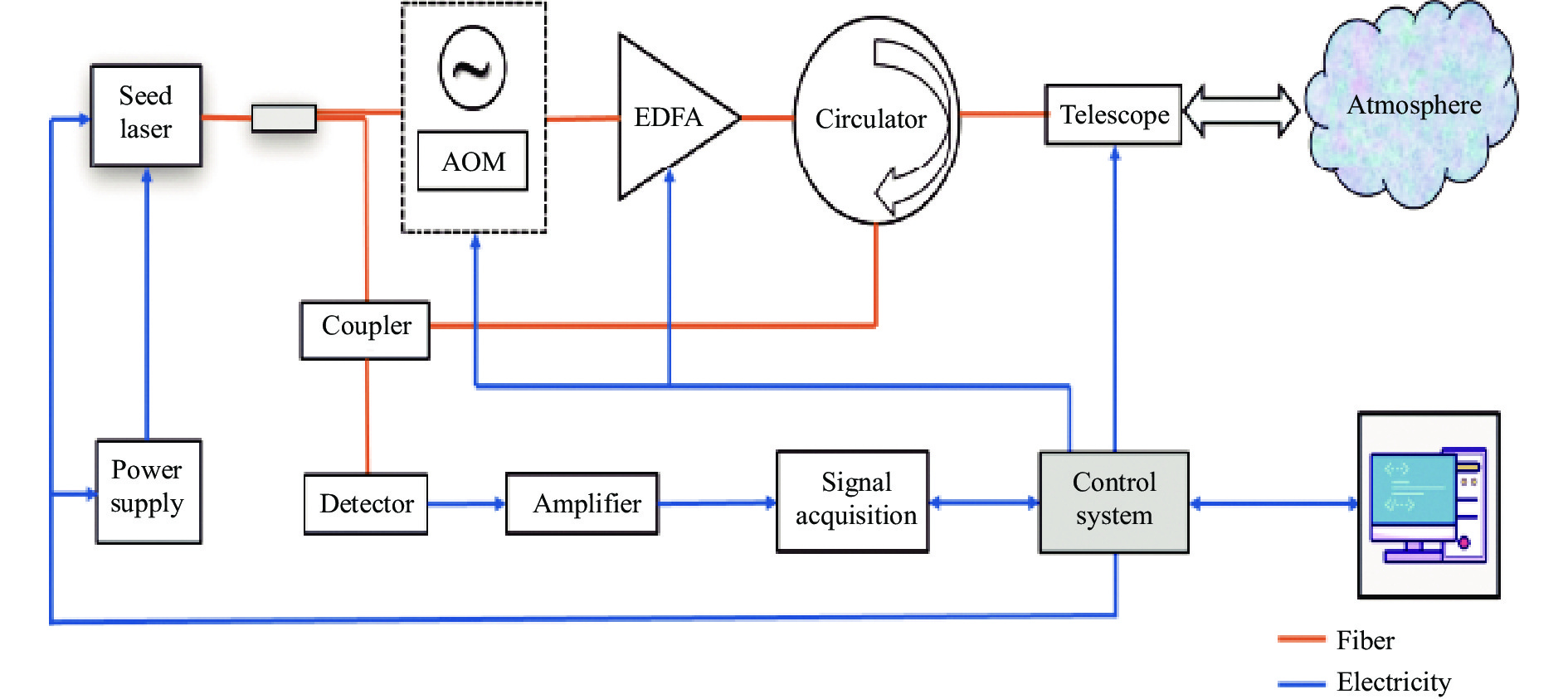
相干激光测风雷达系统组成如图1所示,包括种子激光器、供电系统、探测器、放大器、环行器、光学系统、扫描系统等。其主要工作参数见表1。

图 1 相干激光测风雷达系统组成图
Figure 1. The composition chart of coherent wind lidar
表 1 相干激光测风雷达系统参数
Table 1. System parameters of the coherent wind lidar
Parameter Value Wavelength/μm 1.55 Pulse energy/μJ 150 Pulse repetition rate/kHz 10 Temporal resolution/s ≤1 Range resolution/m 15-200 (adjustable) Wind speed accuracy/m·s–1 0.3 Wind direction accuracy/(°) 3 相干激光测风雷达的回波信号从平衡探测器输出,探测器内信号光与本振光混频后输出的中频电流信号为:
$$ {{I}}_{{RF}}=2\mathfrak{R}\sqrt{{{P}}_{{L}}{{P}}_{{S}}}\mathrm{c}\mathrm{o}\mathrm{s}(2{\pi }{\mathrm{\omega }}_{{d}}{t}+\Delta \mathrm{\varphi }) $$ (1) 式中:$ {P}_{L} $为本振光信号功率,W;$ {P}_{S} $为回波信号功率,W;$ \mathfrak{R} $为探测器响应度,A/W;${\mathrm{\omega }}_{{d}}$为外差频率,Hz;$\Delta \varphi$为本振光和信号光相位差,rad。
电流信号通过探测器阻抗放大转换为电平信号,用于后续处理。探测器输出电平信号为:
$$ {U}_{RF}=2G\mathfrak{R}\sqrt{{P}_{L}{P}_{S}}{\rm{cos}}(2\pi {\omega }_{d}t+\Delta \varphi ) $$ (2) 式中:G为平衡探测器放大倍率,V/A,通常为30×103。则探测器接入信号采集处理板的信号功率PH为:
$$ {P_H} = \frac{{{U_{RF}}^2}}{{{R_L}}} = \frac{{2{P_L}{P_S}{\Re ^2}{G^2}}}{{{R_L}}}{\text{ = }}\frac{{{E_S}{S_R}}}{N}$$ (3) 式中:RL为信号采集处理板阻抗,Ω,通常取50 Ω;ES为采集到的信号能量,J;SR为信号采样率,Hz;N为采样点数。则回波信号功率为:
$$ {P_S} = \frac{{{P_H}{R_L}}}{{2{P_L}{\Re ^2}{G^2}}} = \frac{{{E_S}{S_R}{R_L}}}{{2{P_L}{\Re ^2}{G^2}{{N}}}} = \eta {E_S} $$ (4) 相干激光测风雷达系统最终输出的信号是经过时频转换后的频域信号。根据Parseval定理,时频转换不影响信号能量变化,因此ES=Ef,则可得相干探测系统的回波信号功率:
$$ {P_S} = \eta {E_f} $$ (5) 因此,通过频谱信号计算出信号能量即可得到各距离的回波信号功率,从而用于后续消光系数、云高以及能见度数据的反演计算。
-
相干激光测风雷达方程为:
$$ \begin{split} {P}\left({r}\right)=&{C}\beta \left(r\right){r}^{-2}\mathrm{exp}\left[-{\int }_{0}^{r}2\sigma \left({r}{{'}}\right){\rm{d}}{r}{{'}}\right]=\\& {P}_{0}\frac{c\tau }{2}\frac{{A}_{r}}{{r}^{2}}Y\left(r\right)\beta \left(r\right)\mathrm{e}\mathrm{x}\mathrm{p}\left[-{\int }_{0}^{r}2\sigma \left({r}{{'}}\right){\rm{d}}{r}{{'}}\right] \end{split}$$ (6) 式中:C为激光雷达系统常数;β(r)表示距离r处的后向散射系数,m−1·sr−1;σ(r)表示探测距离r处的大气消光系数,m−1;P0 表示发射功率,J;c表示光速,m/s;τ表示脉冲宽度,s;Ar表示有效接收面积,m2;Y(r)表示激光雷达的几何重叠因子。
对回波信号进行距离平方校准后的数据取对数求微分形式:
$$ \frac{\mathrm{d}{S}\left({r}\right)}{\mathrm{d}{r}}=\frac{1}{\mathrm{\beta }\left({r}\right)}\frac{\mathrm{d}{\beta }}{\mathrm{d}{r}}-2\mathrm{\sigma }\left({r}\right) $$ (7) Klett提出对于弹性散射,假定消光系数与后向散射系数存在如下关系:
$$ \mathrm{\beta }\left({r}\right)={A}{\mathrm{\sigma }\left({r}\right)}^{k} $$ (8) 式中:A为常数;k为消光后向散射对数比,其取决于激光雷达波长和探测的气溶胶性质,通常取值范围为0.67~1.3。则:
$$ \frac{\mathrm{d}{S}\left({r}\right)}{\mathrm{d}{r}}=\frac{{k}}{\mathrm{\sigma }\left({r}\right)}\frac{\mathrm{d}{\sigma }}{\mathrm{d}{r}}-2{\sigma }\left({r}\right) $$ (9) 方程式经Bernoulli方程或Ricatti方程进行处理后,并设k为常数,可求得如下解:
$$ \mathrm{\sigma }\left({r}\right)=\frac{{\rm{exp}}\left\{{\left[S\left(r\right)-S\left({r}_{0}\right)\right]}/{k}\right\}}{{\sigma }^{-1}\left({r}_{0}\right)-{2}/{k}\underset{{r}_{0}}{\overset{r}{\displaystyle\int }}{\rm{exp}}\left\{{\left[S\left({r}{{{'}}}\right)-S\left({r}_{0}\right)\right]}/{k}\right\}{\rm{d}}{r}{{{'}}}} $$ (10) 其中,$ {r}_{0} $和$ \mathrm{\sigma }\left({r}_{0}\right) $通过对$ S\left(r\right) $数据分段线性拟合,并计算出各分段拟合出的线性度$ \delta $进行统计分析,找出$ \delta $最小值即线性度最好的数据认为是均匀分布区域,利用Collis斜率法计算出$ \mathrm{\sigma }\left({r}_{0}\right) $,然后对$ {r\sim r}_{0} $进行后向积分,对$ {r}_{0}\sim r $采用前向积分计算出各距离位置的消光系数$ \mathrm{\sigma }\left(r\right) $。
-
激光雷达云高的算法主要包括阈值法、微分零交叉法、Klett法等[20]。与传统直探激光云高仪原始信号相比,文中采用的收发合一相干激光雷达没有几何重叠因子引起的干扰判断,且回波信噪比强,信号强度随距离变化的噪声干扰小。因此,采用阈值法和微分零交叉法即可识别出云团信息和云高位置,同时与前文通过Klett计算出的消光系数特征值进行综合对比判断,可进一步提高云高数据的质量。
首先,通过阈值法对距离修正后$ S \left(r\right) $的信号分段滑动计算阈值判断选取云团回波强烈的信号。阈值计算采用常规数值统计的计算方法:
$$ thr={S}_{AVR}+k\times \sqrt[]{\sum \frac{{\left(S\right(i)-{S}_{AVR})}^{2}}{n}} $$ (11) 式中:$S \left(i\right)$为各距离的回波强度;$ {S}_{AVR} $为各距离回波强度的平均值,$ {S}_{AVR}={\displaystyle\sum _{0}^{n}S\left(i\right)}/{n} $;k为常数,通常取2~3之间。
判断出有高于阈值$ thr $的信号段$ {r}_{c1} $~$ {r}_{c2} $。利用前文计算出$ {r}_{c1} $~$ {r}_{c2} $位置处的消光系数$\mathrm{\sigma }\left({r}\right)$是否在云团消光阈值$ {\sigma }_{thr} $,若是则判断云团。
最后对$ S\left(r\right) $进行微分:
$$ S'\left(r\right)=\frac{{\rm{d}}S\left(r\right)}{{\rm{d}}r} $$ (12) $ {r}_{c1} $~$ {r}_{c2} $段内S'(r)的零点位置即为云峰位置,m$ {r}_{c1} $~$ {r}_{c2} $前面的零点位置为云底位置,$ {r}_{c1} $~$ {r}_{c2} $后面的零点位置为云顶位置,如图2所示。

图 2 云高算法
Figure 2. Cloud height algorithm
-
在水平大气消光均匀的前提下,气柱的真亮度和大气消光系数均与距离无关近似条件,水平能见度反演方程为:
$$ {V}=-\frac{{\rm{ln}}\varepsilon }{\sigma }=\frac{3.912}{\sigma } $$ (13) 式中:ε为正常人眼的平均亮度对比感阈,通常取0.02;对于其他波长的消光系数需要进行修正。修正公式为${V}=\dfrac{3.912}{\sigma }{\left(\dfrac{550}{\lambda }\right)}^{q}$,其中q通常取经验值如下:
$$ {q}=\left\{\begin{array}{l}0.585{V}^{\tfrac{1}{3}}\qquad V < 6\;{\rm{km}}\\ 1.3 \qquad 6\;{\rm{km}} <V < 50\;{\rm{km}}\\ 1.6\qquad V > 50\;{\rm{km}}\end{array}\right. $$ (14) 当大气消光不均匀时,根据2.1节所述中探测路径上各距离位置的消光系数计算出各距离点的能见度,形成能见度廓线值。对各距离点的能见度进行算数平均可输出探测路径上的平均能见度值。
-
2021年7月,利用银川机场一台三维相干激光测风雷达探测数据与机场内的Vaisala CL31型激光测云仪的数据进行对比验证。数据对比结果如图3所示,激光雷达与激光测云仪测量云高数据基本吻合,相关系数达99.57%,标准偏差为5%,均方根误差为7.2%,充分说明了激光雷达测量云高的可行性及准确性。

图 3 激光雷达和Vaisala云高仪数据对比。 (a) 时序曲线图;(b) 散点图
Figure 3. Comparision of lidar and Vaisala laser-ceilometer cloud height data. (a) Time series diagram; (b) Scatter diagram
-
2021年8月,在成都市温江气象站,利用一台相干激光测风雷达探测的水平能见度数据与气象站能见度仪的数据进行对比验证,数据对比结果如图4所示。激光雷达与能见度仪测量能见度数据趋势一致,相关系数达82.06%,在气象站能见度仪30 km探测范围内,对数据分析得到激光雷达标准偏差精度为12.2%,充分说明了激光雷达测量能见度的可行性及准确性。但是数据分析结果中均方根误差为22.5%,数值较大,可能的原因是:首先,算法中的参数选取不够精确,算法仍存在优化空间;其次,目前相干激光测风雷达系统为单偏振通道探测系统,仍存在信号探测缺陷。针对该问题,后续还需要优化算法以及集成双偏振探测通道系统进行进一步优化。

图 4 激光雷达和能见度仪数据对比。 (a)时序曲线图;(b) 散点图
Figure 4. Comparision of lidar and visibility meter data. (a) Time series diagram; (b) Scatter diagram
-
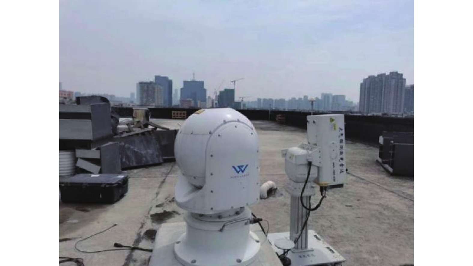
2022年3月~4月,在西南技术物理研究所楼顶,利用1550 nm激光波长的相干激光测风雷达与532 nm激光波长的双偏振气溶胶探测雷达进行了对比试验,试验期间经历晴天、阴天、雨天、雾天等多种气象环境。对比两台激光雷达系统所测量的消光系数,试验现场如图5所示。两台对比设备硬件系统参数对比如表2所示。两种雷达存在较大的差异性,相干激光测风雷达采用1550 nm波长,在测量风场的同时可实现消光系数、云高及能见度的测量,具有无盲区、人眼安全、高灵敏度和高分辨率,同时可达秒级数据获取;气溶胶雷达是基于米散射的直接探测激光雷达,采用532 nm波长测量气溶胶相关参数,可实现消光系数、能见度、PM10、PM2.5气溶胶浓度及退偏比的测量。
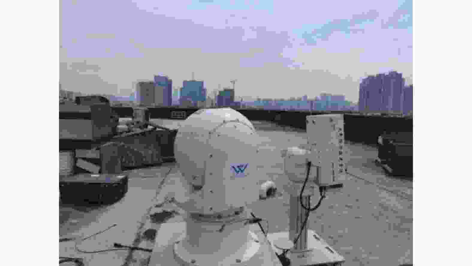
图 5 试验场景
Figure 5. Experimental scene
表 2 相干激光测风雷达和气溶胶雷达系统参数
Table 2. System parameters of the coherent wind lidar and aerosol lidar
System parameter The coherent wind lidar The aerosol lidar Wavelength/nm 1550 532 Detection mode Coherent detection Direct detection Range/km 10 15 Antenna T-R combine, 100 mm T-R separate, 160 mm Pulse energy/μJ 150 20 Pulse repetition rate 10 000 2 000 Data products Wind; Extinction coefficient; Visibility; Aerosol concentration Extinction coefficient; Visibility; PM10 concentration; PM2.5 concentration; Depolarization ratio Advantages No bland zone, without geometric factor correction; Eye-safe; High sensitivity, high time resolution, secondary data acquisition time Visible light, closer to human visibility Disadvantages Invisible light, data conversion required Long acquisition time; Not eye-safe; Bland zone, geometric factor correction required 两种雷达的反演算法也具有各自的优缺点,相干探测激光测风雷达使用改进型Klett算法,利用分段拟合以及标定激光雷达常数等方法查找标定位置进行积分计算消光系数。这种方法算法简单,适用于收发合一的激光雷达,但对标定的激光发射能量和雷达系统常数精度要求很高。气溶胶激光雷达使用Fernald后向积分算法,选取近乎不含大气气溶胶粒子的清洁大气所在的高度为标定高度,利用标准大气模型获得空气分子的密度,再由分子散射理论计算出该处消光系数作为边界值,随后利用边界值进行后向积分计算各距离处消光系数。该方法考虑了大气分子消光系数,计算结果更精确,但是算法复杂,远端边界值难以确定,特别是在有云的天气下容易造成较大测量误差。
下面对两种雷达在各天气条件下探测的结果进行了详细的分析对比。
-
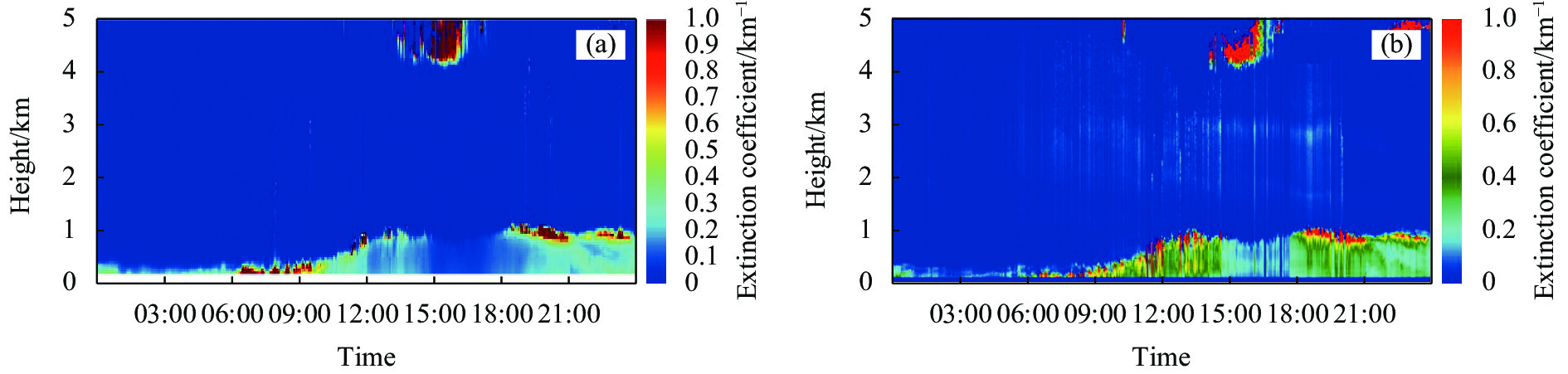
低能见度雾霾天气下,两台设备探测结果一致,包括高空云层位置、厚度,低空消光系数,气溶胶含量随时间变化趋势,以及细节特征等,均比较吻合。消光系数探测对比如图6所示,整个白天能见度较差,云层较低,低空1 km以下从8点半开始能见度差,气溶胶含量高。
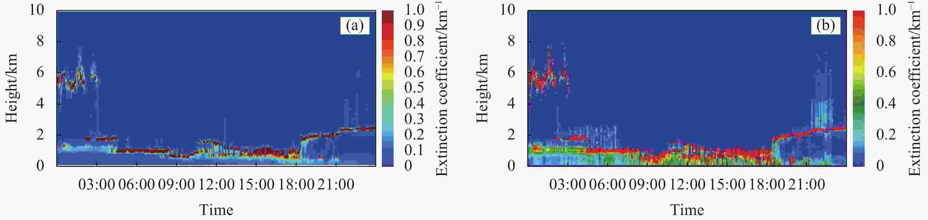
图 6 雾霾天气下消光系数对比。(a) 1550 nm相干激光雷达;(b) 532 nm气溶胶激光雷达
Figure 6. Extinction coefficient comparison in haze day. (a) 1550 nm coherent lidar; (b) 532 nm aerosol lidar
-
晴天高能见度天气下,两台设备探测结果大致一致,均为典型晴天高能见度天气下的低消光系数值。从9点开始,两台低空消光系数探测结果成增加趋势,但1550 nm相干探测雷达探测值增加幅度比较平稳,532 nm气溶胶雷达探测值增加幅度较大,产生的原因可能是两台设备存在差异性,对于该问题还需进一步研究。消光系数探测对比如图7所示。

图 7 晴朗天气下消光系数对比。(a) 1550 nm相干激光雷达;(b) 532 nm气溶胶激光雷达
Figure 7. Extinction coefficient comparison in clear day. (a) 1550 nm coherent lidar; (b) 532 nm aerosol lidar
-
阴转雨天气下,两台设备探测数值与实际天气条件相符,探测数据变化趋势一致,云层探测特征一致。从凌晨至傍晚,低空整体大气结构比较平稳,消光系数变化不大,18点开始气溶胶含量增大,直至21点开始降水。当出现降水时,相干探测雷达出现缺测现象。而气溶胶激光雷达虽然有探测数据,但存在降雨带来的误差,数据可信度不高。相干探测雷达出现缺测的原因主要是雷达镜面积水,激光发射和接收受积水吸收影响而减弱,探测数据也不具备参考性。消光系数探测对比如图8所示。

图 8 阴转雨天气下消光系数对比。(a) 1550 nm相干激光雷达; (b) 532 nm气溶胶激光雷达
Figure 8. Extinction coefficient comparison in overcast and rainy day. (a) 1550 nm coherent lidar; (b) 532 nm aerosol lidar
-
在大雾极低能见度天气下,激光雷达探测距离受到严重影响,两台雷达探测距离受限,严重时不足500 m。特别是在早上大雾时,532 nm气溶胶雷达出现缺测现象。其主要包括两个原因:一是雷达采用收发分离天线方式,存在长达几百米几何重叠区域,该段探测数据没能完全接收到全部激光回波信号,需要进行几何因子校正,若大雾天气下探测距离极低,无法实现该处理方式;二是大雾天气下气溶胶含量太高,532 nm直探式雷达探测达到饱和,无法判断回波信号能量随距离的变化趋势,从而无法反演出数据产品。相反,1550 nm相干探测激光雷达由于采用收发合一天线,几乎无盲区也无需进行几何因子校正,探测器也没有饱和现象,故没有在大雾天气下出现缺测的现象。消光系数探测对比如图9所示。

图 9 大雾天气下消光系数对比。 (a) 1550 nm相干激光雷达;(b) 532 nm气溶胶激光雷达
Figure 9. Extinction coefficient comparison in foggy day. (a) 1550 nm coherent lidar; (b) 532 nm aerosol lidar
-
两台激光雷达消光系数探测结果在大多数天气条件下基本一致,在雨天和大雾等特殊天气条件下由于自身原理性原因出现缺测和数据不准确等现象。
-
结合理论分析及实际探测数据结果,采用相干探测激光雷达进行风场、消光系数、云高及能见度的同时探测,相较于其他直探式的激光雷达气象探测设备将具有更广阔的应用优势。
1)探测效率高、数据探测精度更高。
风场、消光系数、云高、能见度探测的回波信号均为大气中气溶胶散射回波信号,信号光功率往往较弱(大多在pW级)。针对较弱的信号探测,相干探测与直接探测相比具有更高的增益能力。以相干探测与直接探测下的光电探测器输出电功率${{P}}_{{h}}$、${{P}}_{{d}}$进行比较为例:二者的增益比G如公式(15)所示,其中$ {{P}}_{{l}} $、$ {{P}}_{{s}} $分别为本振光和信号光的输出电功率。
$$ G = \frac{{{{{P}}_{{h}}}}}{{{{{P}}_{{d}}}}} = \frac{{2{\Re ^2}{{{P}}_{{l}}}{{{P}}_{{s}}}{R_L}}}{{{\Re ^2}{{{P}}_{{s}}}^2{R_L}}} = \frac{{2{{{P}}_{{l}}}}}{{{{{P}}_{{s}}}}} $$ (15) 假定本振光功率为固定值0.5 mW,当信号光为10−10 W时,增益可达1011,可见相干探测可以大大提高回波信号的探测效率。同时,相干探测还可以抑制杂散光带来的噪声,进一步提高信号提取的精度。
2)与传统气溶胶激光雷达相比,相干激光雷达由于探测效率更高,回波信号信噪比更强,因此采用收发合一的天线结构。该结构形式可消除雷达几何重叠因子,从而简化消光系数、云高等算法,并提高算法计算的准确性。
3)设备高度集成化,数据产品更丰富。单台设备实现多种气象要素的探测,不仅减小了探测系统复杂度,增强了系统稳定性,更有利于机动式探测应用,特别是军事气象保障、环境污染监测等。同时,多种气象要素探测的融合可以产生更丰富的二次数据产品,如风场与气溶胶浓度结合生成气溶胶通量,不仅可以监控污染物的位置、浓度,还可以判断污染物传播方向、速度以及未来运动的态势等。
-
相干激光雷达基于三维相干激光测风雷达,在测量风场的同时实现云高、消光系数及能见度等多种气象要素的探测。文中通过研究相干激光测风雷达信号回波特性,推导出相干激光测风雷达时域回波信号功率的计算方法。利用Klett算法计算出大气消光系数,随后通过阈值法及微分零叉法并综合消光系数反演出云底高度,最后利用消光系数与能见度的关系反演出大气能见度。与云高仪、能见度及气溶胶雷达消光系数的探测对比试验结果表明,1550 nm的相干激光测风雷达具备大气消光系数、云高、能见度探测的能力,云高对比精度可达5.0%,能见度对比精度可达12.2%,探测结果与532 nm的气溶胶激光雷达探测结果具有较高的一致性,并可长期在晴天、阴天、雨天、雾天多种天气环境下连续测量。
Meteorological multi-element detection based on coherent lidar
-
摘要: 相干激光测风雷达具有体积小、探测效率高、信噪比强等特点,在气象、航空保障以及风电等行业得到了广泛的应用,但是目前雷达数据产品大多是利用回波多普勒频移信息反演的风场数据产品,未对雷达回波信号强度信息进行数据挖掘。针对当前相干激光测风雷达数据产品开发不足的问题,介绍了一种新型基于相干探测的激光雷达数据产品生成技术,该技术在探测风场的同时,实现云高、消光系数及能见度等多种气象要素数据产品的生成。首先,通过分析回波信号特性,推导出雷达回波信号功率的计算方法,获取探测范围内各距离位置的回波信号强度信息。在此基础上,利用阈值法和微分零叉法反演出云底高度,同时采用改进型Klett算法实现大气消光系数的反演,继而实现能见度的测量。最后,与气象站能见度仪、激光云高仪以及532 nm气溶胶激光雷达进行数据对比验证试验,试验数据结果显示:云高对比精度可达5.0%,能见度对比精度可达12.2%,消光系数对比有较好的一致性,并可长期在多种气象环境下连续测量。Abstract:
Objective Coherent lidar has the characteristics of small size, high detection efficiency and strong signal-to-noise ratio, and has been widely used in meteorology, aviation and wind power industries. But at present, most coherent wind lidar data products only use echo Doppler frequency shift information to retrieve wind field related products, and do not mine lidar echo signal strength information. Therefore, it is necessary to deeply process the echo signal data of lidar. Methods Considering the insufficient development of the current coherent lidar data products, a new lidar detection technology based on coherent detection was introduced (Fig.1), which can detect various meteorological factors such as cloud height, extinction coefficient and visibility while detecting the wind field. Firstly, by analyzing the characteristics of the echo signal of the coherent wind lidar, the calculation method of the spectrum echo signal power of the coherent wind lidar was derived, and the echo signal strength information of each distance position in the detection range was obtained. Then the differential zero cross and threshold method were used to inverse the cloud bottom height, and the improved Klett method algorithm was used to inverse the atmospheric extinction coefficient, and the visibility measurement was realized. Finally, it was compared with horizontal visibility meter in weather station (Fig.3), laser altimeter (Fig.4) and 532 nm aerosol lidar (Fig.5) for verification. Results and Discussions The results showed that the cloud height, visibility and the extinction coefficient were in good agreement, and lidar can continuously work in various meteorological environments. The cloud height detected by lidar and Vaisala showed that the correlation coefficient is 99.57%, which fully demonstrates the feasibility and accuracy of cloud height by lidar (Fig.3). The standard deviation and root mean square error of lidar are 5% and 7.2% respectively. The trend of visibility data measured by lidar and visibility meter is consistent, and the correlation coefficient is 82.06% (Fig.4). Within 30 km visibility, the accuracy of standard deviation was 12.2%, and root mean square error was 22.5%, which may be due to the following reasons. Firstly, the parameter selection in the algorithm was not accurate enough, and there is still room for optimization in the algorithm; Secondly, at present, the coherent wind radar system was a single polarization channel detection system, which still had signal detection defects. To solve this problem, the optimization algorithm and the integrated dual-polarization detection channel system were needed for further research and optimization. The measurement of extinction coefficient had experienced many meteorological environments such as sunny day, cloudy day, rainy day and foggy day. Extinction coefficient comparison in haze day showed that the results were basically consistent, including the position and thickness of clouds, extinction coefficient, aerosol content and some detailed characteristics (Fig.6). Extinction coefficient comparison in clear day showed that the detection value of coherent lidar increased steadily, while aerosol lidar increased speedily (Fig.7). The reason may be that there are differences between the two devices, which needs further study. Extinction coefficient comparison in overcast and rainy day showed that the detection values of the two devices were consistent with the actual weather conditions. When precipitation occurs, there was a lack of detection by coherent detection lidar. Although aerosol lidar had detection data, it was still unacceptable (Fig.8). Affected by heavy fog, the detection distance of the two lidars were limited, which was less than 500 m. In the morning, the aerosol lidar was missing data in heavy fog, while coherent lidar is still working (Fig.9). There were two main reasons for this phenomenon. First, the geometric factor for the separate antenna mode of transceiver and receiver. Second, in foggy day, the aerosol content was high, and the detection of aerosol lidar reached saturation. Conclusions The results showed that the 1550 nm coherent lidar had the ability to detect atmospheric extinction coefficient, cloud height and visibility. The accuracy of cloud height comparison can reach 5.0%, and the accuracy of visibility comparison can reach 12.2%. The detection results were highly consistent with the detection results of aerosol lidar. It can be measured in sunny, cloudy, rainy and foggy weather continuously. -
Key words:
- lidar /
- meteorological detection /
- coherent detection /
- extinction coefficient /
- visibility /
- cloud height
-
图 3 激光雷达和Vaisala云高仪数据对比。 (a) 时序曲线图;(b) 散点图
Figure 3. Comparision of lidar and Vaisala laser-ceilometer cloud height data. (a) Time series diagram; (b) Scatter diagram
图 4 激光雷达和能见度仪数据对比。 (a)时序曲线图;(b) 散点图
Figure 4. Comparision of lidar and visibility meter data. (a) Time series diagram; (b) Scatter diagram
图 6 雾霾天气下消光系数对比。(a) 1550 nm相干激光雷达;(b) 532 nm气溶胶激光雷达
Figure 6. Extinction coefficient comparison in haze day. (a) 1550 nm coherent lidar; (b) 532 nm aerosol lidar
图 7 晴朗天气下消光系数对比。(a) 1550 nm相干激光雷达;(b) 532 nm气溶胶激光雷达
Figure 7. Extinction coefficient comparison in clear day. (a) 1550 nm coherent lidar; (b) 532 nm aerosol lidar
图 8 阴转雨天气下消光系数对比。(a) 1550 nm相干激光雷达; (b) 532 nm气溶胶激光雷达
Figure 8. Extinction coefficient comparison in overcast and rainy day. (a) 1550 nm coherent lidar; (b) 532 nm aerosol lidar
图 9 大雾天气下消光系数对比。 (a) 1550 nm相干激光雷达;(b) 532 nm气溶胶激光雷达
Figure 9. Extinction coefficient comparison in foggy day. (a) 1550 nm coherent lidar; (b) 532 nm aerosol lidar
表 1 相干激光测风雷达系统参数
Table 1. System parameters of the coherent wind lidar
Parameter Value Wavelength/μm 1.55 Pulse energy/μJ 150 Pulse repetition rate/kHz 10 Temporal resolution/s ≤1 Range resolution/m 15-200 (adjustable) Wind speed accuracy/m·s–1 0.3 Wind direction accuracy/(°) 3  下载: 导出CSV
表 2 相干激光测风雷达和气溶胶雷达系统参数
Table 2. System parameters of the coherent wind lidar and aerosol lidar
System parameter The coherent wind lidar The aerosol lidar Wavelength/nm 1550 532 Detection mode Coherent detection Direct detection Range/km 10 15 Antenna T-R combine, 100 mm T-R separate, 160 mm Pulse energy/μJ 150 20 Pulse repetition rate 10 000 2 000 Data products Wind; Extinction coefficient; Visibility; Aerosol concentration Extinction coefficient; Visibility; PM10 concentration; PM2.5 concentration; Depolarization ratio Advantages No bland zone, without geometric factor correction; Eye-safe; High sensitivity, high time resolution, secondary data acquisition time Visible light, closer to human visibility Disadvantages Invisible light, data conversion required Long acquisition time; Not eye-safe; Bland zone, geometric factor correction required
下载: 导出CSV
-
[1] 周艳宗, 王冲, 刘燕平, 等. 相干测风激光雷达研究进展和应用[J]. 激光与光电子学进展, 2019, 56(2): 020001. Zhou Yanzong, Wang Chong, Liu Yanping, et al. Research progress and application of coherent wind lidar [J]. Laser & Optoelectronics Progress, 2019, 56(2): 020001. (in Chinese) [2] 马福民, 陈涌, 杨泽后, 等. 激光多普勒测风技术最新进展[J]. 激光与光电子学进展, 2019, 56(18): 12. Ma Fumin, Chen Yong, Yang Zehou, et al. Development of laser Doppler wind measurement technology [J]. Laser & Optoelectronics Progress, 2019, 56(18): 180003. (in Chinese) [3] 傅军, 李洁, 吴强. 激光测风雷达在风场观测领域的应用及展望[J]. 空气动力学学报, 2021, 39(4): 172-179. doi: 10.7638/kqdlxxb-2021.0060 Fu Jun, Li Jie, Wu Qiang. Application and prospect of Doppler lidar in the wind field observation [J]. Acta Aerodynamica Sinica, 2021, 39(4): 172-179. (in Chinese) doi: 10.7638/kqdlxxb-2021.0060 [4] 梁晓峰, 张振华. 浅析舰船激光测风雷达技术应用及发展趋势[J]. 激光技术, 2021.45(6): 768-775. doi: 10.7510/jgjs.issn.1001-3806.2021.06.016 Liang Xiaofeng, Zhang Zhenhua. Application and development trend of shipborne wind lidar [J]. Laser Technology, 2021, 45(6): 768-775. (in Chinese) doi: 10.7510/jgjs.issn.1001-3806.2021.06.016 [5] Liang Chen, Wang Chong, Xue Xianghui, et al. Meter-scale and sub-second-resolution coherent Doppler wind LIDAR and hyperfine wind observation [J]. Optics Letters, 2022, 47(13): 3179-3182. doi: 10.1364/OL.465307 [6] 潘静岩, 邬双阳, 刘果, 等. 相干激光测风雷达风场测量技术[J]. 红外与激光工程, 2013, 42(7): 5. doi: 10.3969/j.issn.1007-2276.2013.07.013 Pan Jingyan, Wu Shuangyang, Liu Guo, et al. Wind measurement techniques of coherent wind lidar [J]. Infrared and Laser Engineering, 2013, 42(7): 1720-1724. (in Chinese) doi: 10.3969/j.issn.1007-2276.2013.07.013 [7] 徐冠宇, 尹微, 李策, 等. 相干激光测风雷达高分辨距离门自适应技术研究[J]. 红外与激光工程, 2021, 50(12): 20210187. doi: 10.3788/IRLA20210187 Xu Guanyu, Yin Wei, Li Ce, et al. Research on high resolution range-gate adaptive technology of coherent wind lidar [J]. Infrared and Laser Engineering, 2021, 50(12): 20210187. (in Chinese) doi: 10.3788/IRLA20210187 [8] Krishnamurthy R, Choukulkar A, Calhoun R, et al. Coherent Doppler lidar for wind farm characterization [J]. Wind Energy, 2013, 16(2): 189-206. doi: 10.1002/we.539 [9] Kliebisch O, Uittenbosch H, Thurn J, et al. Coherent Doppler wind lidar with real-time wind processing and low signal-to-noise ratio reconstruction based on a convolutional neural network [J]. Optics Express, 2022, 30(4): 5540-5552. doi: 10.1364/OE.445287 [10] Frehlich R. Coherent Doppler lidar signal covariance including wind shear and wind turbulence [J]. Appl Opt, 1994, 33(27): 6472-6481. doi: 10.1364/AO.33.006472 [11] 靳翔, 宋小全, 刘佳鑫, 等. 基于多普勒激光雷达的边界层内湍流参数估算[J]. 中国激光, 2021.48(11): 111001. Jin Xiang, Song Xiaoquan, Liu Jiaxin, et al. Estimation of turbulence parameters in atmospheric boundary layer based on Doppler lidar [J]. Chinese Journal of Lasers, 2021, 48(11): 1110002. (in Chinese) [12] Jiang Pu, Yuan Jinlong, Wu Kenan, et al. Turbulence detection in the atmospheric boundary layer using coherent Doppler wind lidar and microwave radiometer [J]. Remote Sensing, 2022, 14(12): 2951. doi: 10.3390/rs14122951 [13] Chen Songsheng, Yu Jirong, Mulugeta P, et al. Double-pass Tm:Ho:YLF amplifier at 2.05 μm for spaceborne eye-safe coherent Doppler wind lidar and CO2 differential absorption lidar (DIAL)[C]//Proceedings of SPIE, 2003, 4893: 217-222. [14] Hardesty R M, Brewer W A, Senff C J, et al. Structure of meridional moisture transport over the US Southern Great Plains observed by co-deployed airborne wind and water vapor lidars [C]//Annual Meeting, DLR, 2008. [15] Quan Jiannong, Gao Yang, Zhang Qiang, et al. Evolution of planetary boundary layer under different weather conditions, and its impact on aerosol concentrations [J]. Particuology, 2013, 11(1): 34-40. doi: 10.1016/j.partic.2012.04.005 [16] 董骁, 胡以华, 徐世龙, 等. 不同气溶胶环境中相干激光雷达回波特性[J]. 光学学报, 2018, 38(1): 0101001. doi: 10.3788/AOS201838.0101001 Dong Xiao, Hu Yihua, Xu Shilong, et al. Echoing characteristics of coherent lidar in different aerosol environments [J]. Acta Optica Sinica, 2018, 38(1): 0101001. (in Chinese) doi: 10.3788/AOS201838.0101001 [17] Chouza F, Reitebuch O, Rahm S. Retrieval of aerosol backscatter and vertical wind from airborne coherent Doppler wind lidar measurements [C]//18th Coherent Laser Radar Conference, 2016. [18] Yuan Jinlong, Xia Haiyun, Wei Tianwen, et al. Identifying cloud, precipitation, windshear, and turbulence by deep analysis of the power spectrum of coherent Doppler wind lidar [J]. Optics Express, 2020, 28(25): 37406. doi: 10.1364/OE.412809 [19] 任雍, 陈赛, 余安安, 等. 相干多普勒测风激光雷达反演厦门市风场及边界层高度的可靠性分析[J]. 干旱气象, 2021, 39(3): 514-523. Ren Yong, Chen Sai, Yu Anan, et al. Reliability analysis of wind field and boundary layer height in Xiamen retrieved by coherent Doppler wind lidar [J]. Journal of Arid Meteorology, 2021, 39(3): 514-523. (in Chinese) [20] 张冬冬, 郝明磊, 盛显涛, 等. 基于激光测云仪的云底高反演算法进展研究. 气象水文海洋仪器, 2017, 34(3): 6 Zhang Dongdong, Hao Minglei, Sheng Xiantao, et al. Research on cloud-base height inversion algorithm with laser ceilometers [J]. Meteorological, Hydrological and Marine Instruments, 2017, 34(3): 13-18. (in Chinese) -

 点击查看大图
计量
- 文章访问数: 126
- HTML全文浏览量: 13
- PDF下载量: 46
- 被引次数: 0

