


 下载:
下载:


-
双光子荧光(two-photon fluorescence,TPF)显微成像是实现非线性光学显微成像的重要手段之一,属于三阶非线性光学效应,基于分子振动特性的成像原理可以实现对样品中特定化学元素的成像。凭借其更大的成像深度、更高的空间分辨率与对比度、更小的光漂白性与光损伤,TPF显微成像技术发展成如今新型材料[1]、医药学[2]及生物科学领域的一项重要研究工具。双光子吸收现象于1931年被Göppert-Mayer从理论上提出,并于1961年被Kaiser与Garret在实验中发现。直到1990年,Denk发明了世界上第一台双光子荧光显微镜[3],并对荧光乳胶珠与猪肾细胞的染色体进行了显微成像。经过30多年的发展,TPF显微镜已经发展为一项实用化的技术,尤其是在成像深度与分辨率方面有了长足的进步。
首先,TPF显微成像技术在成像深度以及对活体组织成像方面具有天然的优势,这是因为该技术常采用的近红外波段的激光源刚好处于生物窗口内[4],对生物组织破坏较少[5],穿透性较好[6],使得该成像技术具有较高的成像深度[7-10]。相较于单光子吸收,TPF过程的吸收截面更小,这使得TPF过程的实现需要更高的光子密度,因此,样品只在焦点附近才会被激发[11]。一方面,减小了对生物样品的光漂白性与光毒性,更有利于实现活体生物样品成像[12-13];另一方面,使得TPF显微成像可以实现对较厚组织的不同深度进行断层扫描成像[14],从而对样品进行三维重构,获得样品内部更丰富的信息。
生物医学领域研究的不断深入不仅需要高成像深度并进行活体成像,还对生物细胞结构的研究有着迫切需求,因此,提升TPF显微镜的空间分辨率十分必要。提升成像分辨率最常用的方法是脉冲整形[15]、调整相位分布[16]以及获得更高的激发功率、更窄的脉冲宽度[17]。在2014年,Cheng等人将TPF显微成像的横向分辨率与纵向分辨率分别提高到了168 nm与1.22 μm[18]。另外,多种可以突破衍射极限的超分辨成像技术也应用到TPF显微成像上,例如,随机光学重建显微镜[19]、受激发射损耗[20],结构光照明显微镜[21]。
文中利用飞秒激光器作为激发光源,搭建了TPF显微成像系统。使用该系统测量了罗丹明B溶液的TPF光谱,实现了对罗丹明B染色的小鼠大脑切片的激发,开展了小鼠大脑切片的断层扫描成像与三维重构实验。在实验中采用主客观分析相结合的研究方法,通过对三维图像的观测后再对样品关键部位的荧光强度分布进行分析,可以快速锁定研究区域。在以往的成像研究中常采用直接观察图像并结合光谱的方法对样品中特定细胞或组织进行定性的分析,却少有研究通过处理强度分布数据来对样品的关键部位进行定量的分析。文中利用该方法获得了小鼠大脑灰质与白质两种不同组织的分布与结构信息,有助于研究哺乳动物大脑的微观结构以及神经元作用机制。还测得了成像系统的横向分辨率与成像深度等参数。
-
由于双光子吸收过程属于非线性光学效应,吸收的光子数与光强并非线性关系,而是与光强I的平方成正比,与吸收截面δ成正比。而单光子吸收过程则不属于非线性光学效应,荧光光强与激发光强成线性关系。通过推导双光子荧光的空间分布公式来研究TPF显微成像的成像深度与分辨率。定义光斑半径为ω,束腰处的光斑半径为ω0,瑞利距离为$z_0 $,激发光的波长为λ。以激光的传播方向为轴,以束腰为中心建立柱坐标系,任意一点与光轴的距离为r,与中心的轴向距离$z $。高斯光束复振幅的空间分布可以表示为:
$$ E\left(r,z\right) = {E}_{0}\frac{{\omega }_{0}}{\omega \left(z\right)}\times \mathrm{exp}\left[ -\frac{{r}^{2}}{{\omega }^{2}\left(z\right)} \right]\times \mathrm{e}\mathrm{x}\mathrm{p}\left[ -ik\left(z+ \frac{{r}^{2}}{2R(z)}-\phi (z)\right) \right] $$ (1) 式中:E0为光束中心的复振幅;${\omega }\left(z\right) $表示沿轴方向各位置光斑大小。
$$ {\omega }^{2}\left(z\right)={\omega }_{0}^{2}\left[1+{\left(\frac{z}{{z}_{0}}\right)}^{2}\right] $$ (2) $$ {z}_{0}=\frac{\pi }{2}{\omega }_{0}^{2} $$ (3) 从公式(1)中可以看出,公式分为三部分,第一项与第二项为振幅衰减因子,最后一项为相位衰减因子。任意位置的振幅大小可以通过将该位置的深度以及与光轴的距离代入公式(1)来确定。
光强的大小为复振幅的平方,因此荧光光强的公式表示为:
$$ I={E}_{0}^{2}\frac{{\omega }_{0}^{2}}{{\omega }^{2}\left(z\right)}\mathrm{e}\mathrm{x}\mathrm{p}\left(-\frac{2{r}^{2}}{{\omega }^{2}\left(z\right)}\right) $$ (4) 将E02替换为I0,得到:
$$ I={I}_{0}\frac{{\omega }_{0}^{2}}{{\omega }^{2}\left(z\right)}\mathrm{e}\mathrm{x}\mathrm{p}\left(-\frac{2{r}^{2}}{{\omega }^{2}\left(z\right)}\right) $$ (5) 由于TPF的荧光强度则与激发光的平方成正比。因此TPF的荧光强度分布为:
$$ {I}_{\mathrm{T}\mathrm{P}\mathrm{M}}={A}{I}_{0}^{2}\frac{{\omega }_{0}^{4}}{{\omega }^{4}\left(z\right)}\mathrm{e}\mathrm{x}\mathrm{p}\left(-\frac{4{r}^{2}}{{\omega }^{2}\left(z\right)}\right) $$ (6) 式中:A为TPF激发光强度的平方的比例系数。若要得到TPF信号强度的轴向分布,应忽略位置与光轴的距离r的影响,仅考虑位置与中心的轴向距离$z $,这里令r=0,得到:
$$ {I}_{\mathrm{T}\mathrm{P}\mathrm{M}-{z}}={A}{I}_{0}^{2}\frac{{\omega }_{0}^{4}}{{\omega }^{4}\left(z\right)} $$ (7) 通过公式(7)可以看出,TPF信号强度轴向分布的特点。在轴向任意深度处的TPF信号强度与总光强的平方成正比,与激光的束腰半径的四次方成正比,而与在该深度下的光斑大小的四次方成反比。在成像深度为0时,TPF信号强度均为最大值。随着位置沿$z $轴向两边移动,荧光强度逐渐减小。
如果仅考虑位置与光轴的距离r的影响,可以得到单光子荧光和TPF信号的径向分布。令$z $=0,因此${\omega }\left(z\right) $=ω0,得到:
$$ {I}_{\mathrm{T}\mathrm{P}\mathrm{M}-{r}}={A}{I}_{0}^{2}\mathrm{e}\mathrm{x}\mathrm{p}\left(-\frac{4{r}^{2}}{{\omega }^{2}\left(z\right)}\right) $$ (8) 通过公式(8)可以看出TPF信号强度的径向分布不仅与距离r有关,还受到此处的光斑大小${\omega }\left(z\right) $的影响。在确定深度下,平面上某点的TPF信号强度与总光强的平方成正比,并且随着距离r的增加,该点的信号强度随r2呈e指数衰减。而在不同深度下,光斑越大,则信号强度随距离r的增加衰减得更快。
-
公式(5)~(8)为理想情况下高斯光束的单光子荧光与TPF信号的强度分布,然而对较厚的生物样品进行显微成像时,组织对光会有吸收与散射效应。对于近红外光源,组织对光的吸收效应相较于散射效应十分微弱,可以忽略。只有非散射光子才能到达物镜,被探测仪器采集,称为弹道光子,弹道光子数量随着成像深度的增加呈指数衰减。入射光强与深度$z $的关系为:
$$ {I}_{\mathrm{T}\mathrm{P}\mathrm{M}-{r}}=\mathrm{A}{I}_{0}^{2}\mathrm{e}\mathrm{x}\mathrm{p}\left(-\frac{4{r}^{2}}{{\omega }^{2}\left(z\right)}\right) $$ (9) 定义lex为激发光在组织中的散射长度,并且TPF的荧光强度与激发光的平方成正比。则:
$$ {I}_{\mathrm{T}\mathrm{P}\mathrm{M}}={\mathrm{A}I}_{0}^{2}\mathrm{e}\mathrm{x}\mathrm{p}\left(-\frac{2z}{{l}_{\mathrm{e}\mathrm{x}}}\right) $$ (10) $z $的方向以深入样品为正,散射效应只发生在样品内部,因此公式(10)在$z $>0时成立。根据公式(9)可以得到的最大成像深度${z}_{\mathrm{m}\mathrm{a}\mathrm{x}} $为:
$$ {z}_{\mathrm{m}\mathrm{a}\mathrm{x}}={l}_{\mathrm{e}\mathrm{x}}\mathrm{l}\mathrm{n}\left[{I}_{0}\sqrt{\eta \varphi }\sqrt{1/f\tau }\right] $$ (11) 式中:η为荧光量子效率;φ为荧光收集效率;f与τ为激发光脉冲的重复频率与脉冲宽度。从公式(11)中可以看出,增加激光器的输出功率、以及减小脉冲的重复频率与脉冲宽度都可以增加TPF的成像深度。
-
在1.2节中已经推导出TPF信号强度的径向分布公式(8),得到了光强在样品的X~Y平面上的分布情况。激光器输出的光束为高斯光束,束腰位置的光斑最小。光斑大小为光强衰减为中心光强的e−2时的宽度,成像时两像素点之间的距离应不小于2ω0。因此TPF的横向分辨率为:
$$ {r}_{\mathrm{T}\mathrm{P}\mathrm{M}-{x}{y}}=2{\omega }_{0}=2\frac{\lambda {f}_{0}}{\pi \omega } $$ (12) 式中:λ为激发光的波长;ω为光束在物镜前的光斑大小。又因为:
$$ \frac{{f}_{0}}{\omega }=\mathrm{c}\mathrm{o}\mathrm{t}\alpha $$ (13) 式中:α为物镜的汇聚角。将公式(12)改写为:
$$ {r}_{\mathrm{T}\mathrm{P}\mathrm{M}-{x}{y}}=2\frac{\lambda }{\pi }\frac{\sqrt{1-{\mathrm{s}\mathrm{i}\mathrm{n}}^{2}\alpha }}{\mathrm{s}\mathrm{i}\mathrm{n}\alpha } $$ (14) 在实验中,很难去测量光束的汇聚角,但是往往物镜的数值孔径NA是已知的,NA=n·sinα,其中n为物镜与样品之间介质的折射率。对于普通物镜,介质为空气,此时n=1。对于油浸物镜,此时n=1.5。将数值孔径NA代入公式(14)中,得到:
$$ {r}_{\mathrm{T}\mathrm{P}\mathrm{M}-{x}{y}}=2\frac{\lambda }{\mathrm{\pi }}\frac{\sqrt{{n}^{2}-{NA}^{2}}}{NA} $$ (15) Zipfel等人根据高数值孔径衍射理论拟合出TPF显微成像的分辨率公式[11],根据纵向分辨率rTPM-z为光照点扩散函数的平方(IPSF2)纵向极限的1/e,横向分辨率rTPM-xy为IPSF2纵向极限的1/e,得到TPF显微成像的纵向与横向分辨率为:
$$ {r}_{\mathrm{T}\mathrm{P}\mathrm{M}-{z}}=\frac{0.532\sqrt{2\mathrm{l}\mathrm{n}2}\lambda }{n-\sqrt{{n}^{2}-{NA}^{2}}} $$ (16) $$ {r}_{\mathrm{T}\mathrm{P}\mathrm{M}-{x}{y}}=\frac{0.320\sqrt{2\mathrm{l}\mathrm{n}2}\lambda }{NA} $$ (17) 式中:NA为物镜的数值孔径。公式(17)为NA大于0.7时的横向分辨率,而NA小于0.7时的横向分辨率公式为:
$$ {r}_{\mathrm{T}\mathrm{P}\mathrm{M}-{x}{y}}=\frac{0.325\sqrt{2\mathrm{l}\mathrm{n}2}\lambda }{{NA}^{0.91}} $$ (18) 该实验使用物镜的数值孔径NA为0.65,可以计算出显微成像系统的横向分辨率理论上为453 nm,纵向分辨率为2.087 μm。
-
实验中搭建的TPF显微成像系统如图1所示。包括准直光路、扫描光路、光谱测量光路、显微成像和信号采集的装置。系统的激发光源采用钛蓝石飞秒激光器(Spectra-Physics,Mai Tai),输出光的中心波长在800 nm,重复频率为80 MHz,脉宽为100 fs。

图 1 TPF显微成像以及TPF光谱系统。BS:分束片;L3、L4、SL、TL:透镜;GM:扫描振镜;OBJ:物镜;M:反射镜;F:滤波片;PMT:光电倍增管;PC:计算机
Figure 1. TPF microscopic imaging as well as TPF spectroscopy system. BS: beam splitter; L3, L4, SL, TL: lens; GM: scanning oscillator; OBJ: objective; M: reflector; F: filter; PMT: photomultiplier tube; PC: computer
在需要测量荧光光谱时选择性地放置二向色镜,一部分激光经过分束片的反射进入到TPF光谱测量系统。透镜L1的焦距为40 mm,将激发光聚焦到装有样品液体溶液的比色皿上,以此激发样品产生TPF信号。使用光谱仪(Andor,Kymera 328i-B2)测量荧光光谱,焦距为50 mm的透镜L2在侧面将荧光信号聚焦到光纤头上采集TPF信号,以减少激发光等背景的干扰。并由光谱仪中的ICCD在−25 ℃下进行探测,在控制电脑上观测和记录。
皮秒脉冲光经分束片入射至显微成像系统,首先通过焦距分别为125 mm与75 mm的两个透镜L3与L4进行缩束。使用X-Y二维扫描振镜GM (Thorlabs,GVSM002/M)对光束进行偏转,从而实现对二维图像的扫描。通过焦距为100 mm的扫描透镜SL聚焦光束,并送入倒置显微镜中(Olympus,IX71)。激光从显微镜入口中心处进入,透过二向色镜和焦距为175 mm管透镜TL到达物镜。显微镜的物镜(UPlanSApo),将光束紧聚焦到样品表面。样品固定于二维位移平台上,通过电驱动的方式改变成像位置。激发出的荧光经二向色镜反射后,入射到带通滤波片F上(Boson,675/67),滤除荧光信号以外的成分。使用PMT (Hamamatsu,R3896)采集信号,将荧光信号转换为电信号并放大,再由电脑处理得到显微成像结果,得到大小为1000 pixel×1000 pixel的图像,系统所需时间约为5 s。
-
罗丹明B的化学式为C28H31ClN2O3,是一种呈暗紫色粉末的人工合成的染料,易溶于水、乙醇,微溶于盐酸和氢氧化钠等溶液。水溶液为蓝红色。罗丹明B样品具有高荧光特性,稳定性好、消光系数大、荧光量子产率高、发射波长较长、毒性低、水溶性好,因此是荧光显微成像实验的常用染料。
在开展对小鼠大脑切片的显微成像实验之前,需要测量罗丹明B染色剂的荧光光谱。在配置罗丹明B溶液时,使用无水乙醇作为溶液。取少量罗丹明B粉末加到容器中,滴加无水乙醇直至固体粉末完全溶解。从容器中取适量的罗丹明B溶液到比色皿中,用于罗丹明B的光谱测量实验。使用比色皿测量光谱不仅可以让样品更均匀地激发,而且更便于收集荧光信号。
图2(a)为飞秒激光器的光谱图,图2(b)为罗丹明B的TPF光谱图,光谱强度经过归一化处理。从图中可以看出,飞秒激光器的中心波长为800 nm,光谱半高宽为14.47 nm。荧光的光谱范围覆盖从610~690 nm,强度从620 nm处开始陡峭地上升,在630 nm出现峰值,之后随波长增加强度缓慢下降,因此飞秒激光器可以有效地激发样品的TPF信号。在后续成像实验中,选用中心波长在675 nm的带通滤波片,带宽为67 nm。TPF显微成像的探测窗口如图2(b)中的虚线框所示,覆盖636~703 nm的范围,此范围可以包含TPF信号的大部分波长范围,尤其是光谱中长波长部分。

图 2 (a) 飞秒激光器的光谱图;(b) 罗丹明B的荧光光谱图
Figure 2. (a) Spectra of femtosecond laser; (b) Fluorescence spectra of rhodamine B
-
小鼠大脑与人脑在神经元与受体的结构、神经递质等方面有着较高的相似性,小鼠的认知习惯、行为模式与人类有诸多共通性。并且小鼠生长周期短,价格便宜,已经成为神经科学与显微成像领域的重要研究素材。因此,文中实验选择罗丹明B染色的小鼠脑组织切片作为研究样品。
在成像时,将样品放置于电动平台上,盖玻片的一面朝向物镜。先粗调焦距再细调焦距直到视野内图像最清晰。移动电动平台,选择有辨识度的成像区域。在成像时,应先选择较低的增益档位,逐渐增加电压直到图像清晰,避免PMT的电流过大使图像过曝。实际操作中影响实验结果的因素有多种,尤其是扫描光路的搭建。缩束准直光路可以缩小光斑直径,提高光束质量。过大的光斑直径不利于能量集中,导致激发功率的降低,然而光斑直径小于物镜的通光孔径,则不利于成像分辨率的提升,因此应选择合适的光斑直径。准直后的光束应入射到X轴扫描振镜的正中心,避免扫描区域的偏移。同时Y轴扫描振镜、扫描透镜与显微镜入口三者的中心应在同一水平轴上。光束斜入射显微镜的入口,会导致荧光偏离光路,无法被PMT所采集。
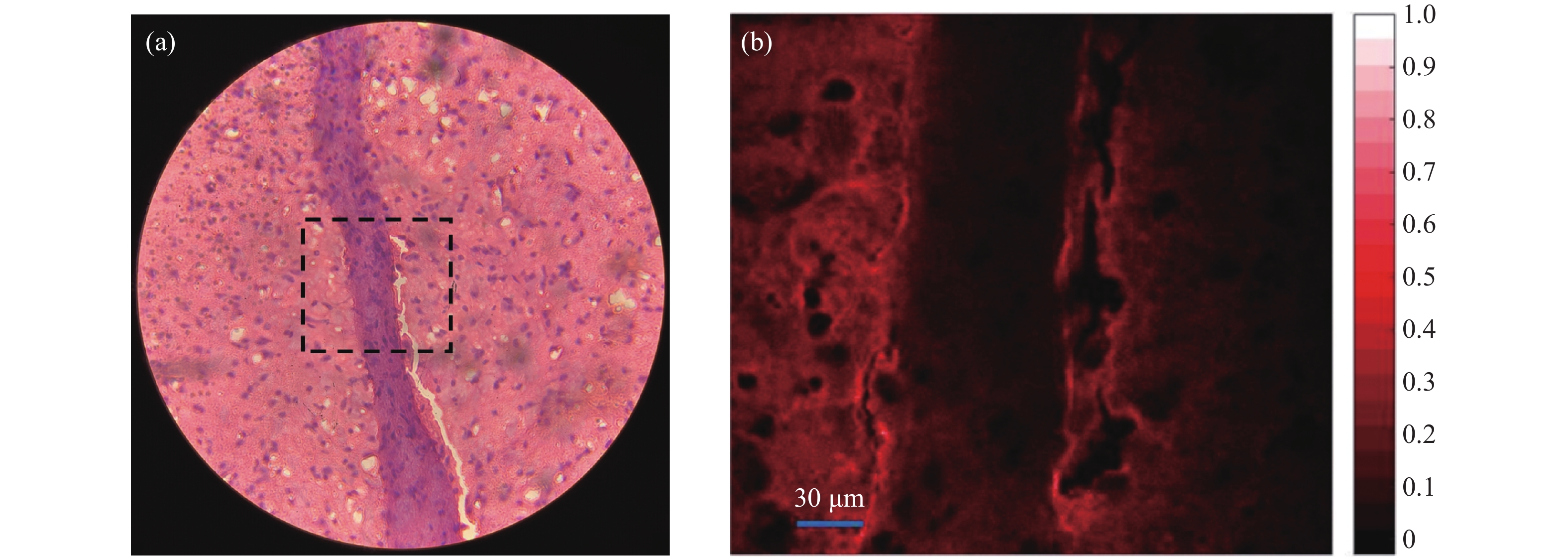
透过显微镜目镜观察到的小鼠大脑细胞如图3(a)所示,其中浅色部分主要为神经纤维的细胞质,称为白质。而神经纤维的细胞体内含有细胞核,颜色较深,称为灰质。成像区域的大小为300 μm×300 μm。对虚线框内的区域进行成像,PMT施加的电压大小约为800 V。原图像大小为1000 pixel×1000 pixel,由于采用“之”字型的扫描线路,图像边缘包含重复扫描的内容,截去边缘后的900 pixel×900 pixel的显微成像结果如图3(b)所示。由于振镜的扫描顺序以及光路结构的原因,图3(b)为图3(a)经过上下翻转与左右翻转后的结果。图中颜色的深浅代表荧光强度的大小,白色部分代表图中荧光最强的区域,图右侧数值为对应颜色的荧光强度。可以看出,荧光强度分布状况可以清晰反映生物组织的结构信息。并且灰质的荧光强度较弱,而白质则具有更高的荧光强度。

图 3 (a) 小鼠大脑切片的成像区域(虚线框内);(b) 小鼠大脑切片的TPF显微成像结果
Figure 3. (a) Imaging area of mouse brain (in dashed box); (b) TPF microscopic image of a mouse brain slice
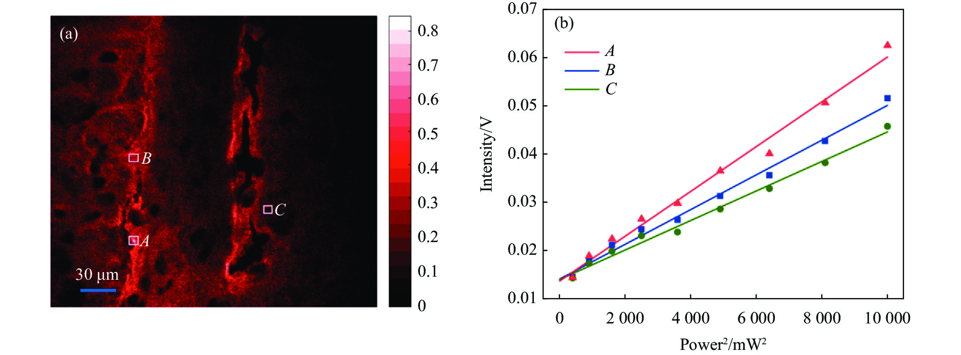
为了定量地研究荧光强度与激发功率之间的关系,调节可变衰减片使显微镜入口处的功率从10~100 mW,间隔10 mW。在不同功率下对同一区域进行TPF显微成像。选取成像结果中三个不同浓度的区域,对应图4(a)白色方框区,范围大小均为25 pixel×25 pixel。对于罗丹明B浓度,区域A>区域B>区域C。反映到成像结果上,区域A亮度最大,区域C亮度最小。对三块区域内荧光强度取平均值,荧光强度与激发光功率平方的变化趋势如图4(b)所示。其中红色三角代表区域A,蓝色方块代表区域B,绿色圆形代表区域C。利用一次函数拟合三个目标区域平均荧光强度的变化,红色直线、蓝色直线、绿色直线分别代表区域A、B、C的激发功率平方与荧光强度的变化关系。

图 4 (a) 小鼠大脑在100 mW激发功率下的TPF成像图;(b) A、B、C三块不同浓度区域(白色方框内)平均荧光强度随激发功率平方变化趋势
Figure 4. (a) TPF imaging plot of mouse brain at 100 mW excitation power; (b) The trend of average fluorescence intensity with power squared for the regions of A, B, C (inside the blue box)
可以看出三块区域具有相似的变化趋势,随着激发功率的提升,TPF信号均有明显的升高。激发功率越大,三块区域的荧光强度相差越大。而在较低的激发功率下,三块区域有着近似的荧光强度,这是因为在低功率激发下图像的噪声掩盖了荧光信号。数据点近似地分布在拟合直线附近,可以有效说明荧光强度与激发功率的平方呈线性关系,证明了成像系统采集到的是TPF信号。
为了得到小鼠大脑组织的内部构造,使用800 nm激发光对样品进行三维重构实验。从样品表面到14 μm深度范围内对样品沿Z轴进行断层扫描成像,每采集一次图像向下移动1 μm的距离。成像结果如图5所示,图5(a)为生物样品表面的成像图以及沿白色虚线的剖面图,图5(b)为沿Y轴的剖面图。
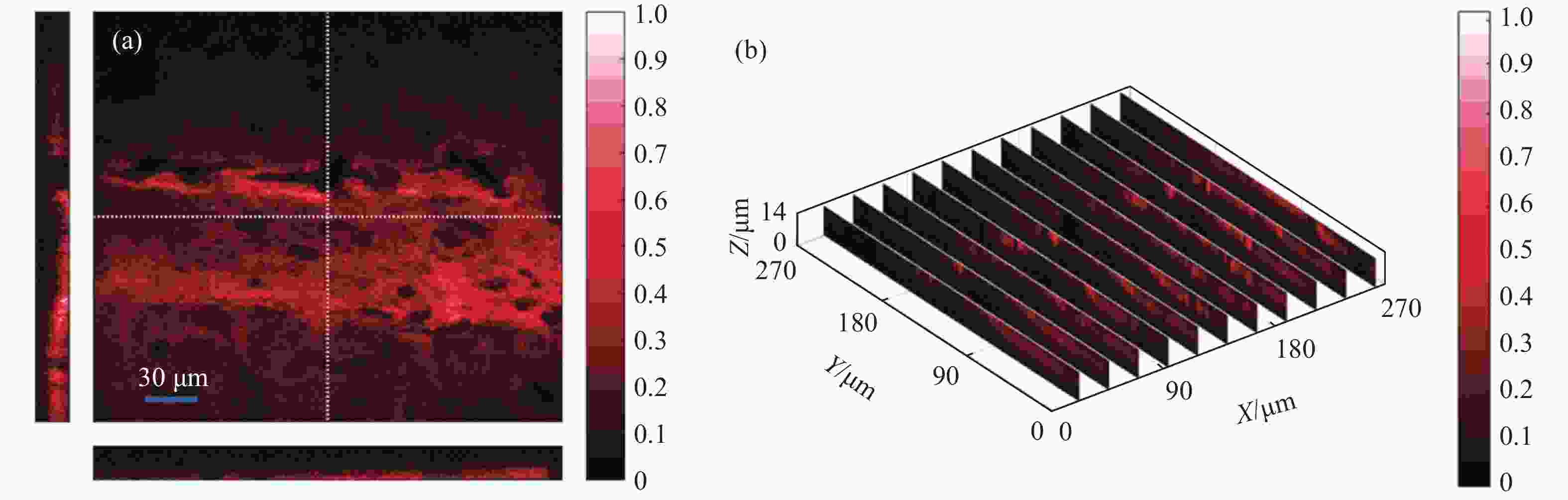
图 5 (a) 小鼠大脑的断层扫描成像结果;(b) 小鼠大脑沿Y轴的剖面图
Figure 5. (a) Tomography imaging of mouse brain; (b) Imaging results of mouse brain slice along the Y-axis
通过对TPF成像结果的分析发现,在沿Z轴向下扫描成像的过程中,从0~4 μm的深度范围内图像的整体亮度逐渐提升,在4 μm处达到最高。从5 μm开始图像的整体亮度快速下降,在14 μm处图像整体亮度降为最高处的1/4。然而生物样品不同于化学样品,其内部构造复杂,存在许多微小结构,因此无法简单地用图像整体亮度来反映内部物质分布状况。
样品在0、2、4、6、8、10 μm深度的TPF显微成像图如图6所示。从图中可以看出,在样品表面,小鼠大脑的灰质部分相较于白质的荧光强度更高。随着深度的增加,灰质部分的荧光强度逐渐减弱,而白质部分的荧光强度开始增加。在3 μm的深度,小鼠大脑白质的荧光强度开始高于灰质部分。在6 μm的深度,灰质部分的荧光信号几乎消失,强度仅为白质部分的1/18。受限于系统的成像深度,深度继续增加,小鼠大脑白质的荧光信号逐渐减弱。

图 6 (a)~(f) 小鼠大脑在0、2、4、6、8、10 μm深度的TPF显微成像结果
Figure 6. (a)-(f) TPF microscopy results of mouse brain at 0 μm, 2 μm, 4 μm, 6 μm, 8 μm, and 10 μm
小鼠大脑的成像结果表明,灰质相比于白质有着更高的荧光效率,并且小鼠大脑切片的灰质只存在样品浅层,而白质部分厚度更大。目前,大多数关于小鼠大脑的TPF显微成像研究中主要通过分析图像获得样品的信息。为了更客观地分析小鼠大脑样品中不同组织的分布情况,实验部分采用对显微图像与样品关键部位强度分布分析相结合的研究方法。首先在灰质与白质区域各取一列数据,对比荧光强度的分布情况。图7为小鼠大脑图像的第400列(灰质)与第200列(白质)数据在0、3、6、9 μm深度的荧光强度分布曲线。图的横坐标为像素位置,纵坐标为该像素点的PMT电信号的电压。

图 7 (a) 小鼠大脑灰质在不同深度的强度分布曲线;(b) 小鼠大脑白质在不同深度的强度分布曲线
Figure 7. (a) Intensity distribution curves of mouse brain gray matter at different depths; (b) Intensity distribution curves of mouse brain white matter at different depths
通过分析强度分布曲线可以得出,灰质部分在样品表面的荧光强度最高,较白质部分高出50.1%,随着深度的增加而减弱,在9 μm的深度强度降为表面的1/9.8。因此,灰质荧光效率比白质更高,并且存在于样品的浅层部分。白质部分在表面的荧光强度相对较低,在3 μm和6 μm的深度荧光强度有所提升,在5 μm的深度平均强度达到最高,为表面的2.4倍。白质部分在9 μm深度的平均荧光强度降到最高的1/3.6,但仍比同深度的灰质高出3.3倍。可以看出小鼠大脑切片的白质较深,纵向分布更广。强度曲线的分析结果与TPF显微成像结果相符。
在三维显微成像实验中,图像的深度间隔为1 μm,因此无法精准测量成像深度。为了获得样品的荧光强度的纵向分布情况,分别在小鼠大脑的灰质与白质部分取大小为25×25像素点的区域,计算区域内的平均荧光强度。图8为使用算法拟合得到的小鼠大脑灰质与白质的平均荧光强度随深度变化曲线。

图 8 小鼠大脑的灰质与白质组织的平均荧光强度随深度变化曲线
Figure 8. Average fluorescence intensity changing curves with depth in gray and white matter tissue of mouse brain
图8的横坐标为成像时的深度,纵坐标为归一化的荧光强度。从图中可以看出:在样品表面处灰质的荧光强度要高于白质部分,随着深度的增加,白质部分的荧光强度逐渐增强,在1.5 μm深度达到最大,强度分布曲线与图像观察结果基本相符。经过计算灰质与白质荧光强度分布曲线分别在10.1 μm与12.9 μm深度时斜率变为0,说明深度大于12.9 μm后,成像系统仅能采集到噪声,因此,成像系统的成像深度达到了12.9 μm。通过公式(11)得知在光源参数相同的情况下,影响成像深度的主要因素为散射长度lex。由于灰质组织比白质组织密度更大,lex更小,激光在表层的灰质组织后受到的散射效应更强,因此,灰质区域的成像深度较小。
从图3(a)中可以看出,小鼠大脑切片样品中存在多处不含组织细胞的狭窄缝隙,通过显微成像来寻找能够分辨的最小距离,就可以得出成像系统分辨率的大小。从成像结果中横向选取的四处含有缝隙的100个连续像素点,如图9所示,分别为D、E、F、J,结果图中100 pixel对应30 μm。分别绘制四处的强度分布曲线,如图10所示,曲线中凹陷部分对应样品的缝隙位置。分析凹陷部分的半高宽,数值最小的宽度即为成像系统的分辨率。
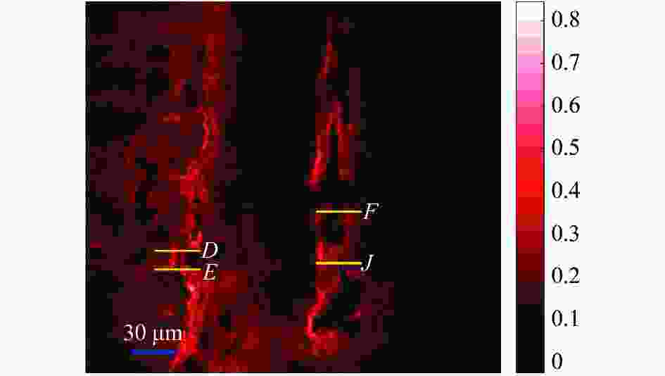
图 9 在小鼠大脑切片上横向选取的四处含有缝隙的100个连续像素点
Figure 9. Four consecutive 100 pixels with gaps of the mouse brain samples

图 10 小鼠大脑成像结果中四条线段的强度分布曲线
Figure 10. Intensity distribution curves of four lines in mouse brain imaging
从图10中可以看出,线段D的宽度为8 pixel,对应2.4 μm。线段E的宽度为7.5 pixel,对应2.25 μm。线段F的宽度为19 pixel,对应5.7 μm。线段J的宽度为10 pixel,对应3 μm。其中线段E的宽度最小,可认为成像系统的横向分辨率至少为2.25 μm。由于样品中不存在间距刚好为最小分辨率的缝隙,借此方法得到的分辨率数值要大于理论计算的453 nm。如果存在能够清晰分辨的更窄缝隙,则可以测出更加精准的分辨率数值,从而更加接近理想分辨率。
-
文中介绍了搭建的TPF显微成像系统,使用飞秒锁模激光器作为激发光源。在800 nm波长的激发下,测量了罗丹明B溶液样品的荧光光谱。光谱范围覆盖从610~690 nm,峰值出现在630 nm,因此为后续显微成像实验选择了636~703 nm的探测窗口。开展了罗丹明B染色的小鼠大脑切片的TPF显微成像实验,通过断层扫描成像,获得生物样品在0~14 μm深度内的荧光强度分布。经过对图像的三维重构,得出小鼠大脑样品内灰质部分位于样品6 μm以内的浅层,而白质部分纵向分布更广,并且小鼠大脑灰质的荧光强度更高,具有比白质部分更高的密度。同时文中对样品关键部位的荧光强度数据进行分析,得出显微成像系统的成像深度为12.9 μm,以及系统的横向分辨率至少小于2.25 μm。显微成像系统生产一张1000 pixel×1000 pixel的图像所需时间约为5 s。
Two-photon fluorescence 3D microscopic imaging of mouse brain based on femtosecond pulses
-
摘要: 双光子荧光(two-photon fluorescence,TPF)显微成像技术借助荧光探针实现样品中被标记成分的特异性成像,具有天然的三维层析能力、高成像深度与空间分辨率、以及更小的光漂白与光损伤,已经发展成为化学、医药学和生命科学领域的一项重要研究工具。文中通过分析高斯光束复振幅在空间中的分布,推导出TPF信号的纵向与径向分布公式,以此估算出文中的TPF显微成像系统的横向分辨率为453 nm,纵向分辨率为2.087 μm。使用飞秒激光器作为激发光源,搭建了TPF显微成像系统。在800 nm波长的飞秒脉冲激发下,测量了罗丹明B溶液的TPF光谱,从而选择636~703 nm作为显微成像的荧光探测窗口。随后开展了对罗丹明B染色的小鼠大脑切片的TPF显微成像实验研究,利用断层扫描成像的方式获得了小鼠大脑切片在0~14 μm深度内的荧光强度分布。通过三维重构完成了对生物样品的三维立体成像,获得了小鼠大脑中灰质与白质在不同深度的分布情况,实验结果证明了搭建的显微成像系统具有优异的成像深度与空间分辨能力。Abstract:
Objective Optical microscopy technology is to observe and record images of the microstructure of objects at a scale indistinguishable from the human eye, and has become an important tool for human observation of the microscopic world. Among them, electron microscopy has a resolution that breaks the limit of optical diffraction and can reach the nanometer level. However, it needs to provide a vacuum environment for electron acceleration, so it is not conducive to the observation of living samples. Optical microscopes are easy to operate and inexpensive, and are widely used in scientific research, industry, medicine and other fields. Conventional light microscopes rely on the contrast produced by differences in the optical properties of the sample for imaging, and do not require labeling or staining, but do not have sufficient specificity. In contrast, nonlinear optical microscopy not only realizes specificity imaging, but also has higher imaging depth and resolution. Among them, fluorescence microscopy technology with the help of fluorescent probes to label different components within the biological sample, through the detection of fluorescence signal to achieve imaging of the labeled components in the sample, to obtain its distribution within the sample. TPF (two-photon fluorescence) microscopic imaging technology based on the nonlinear effect of two-photon absorption, the fluorescence signal will not be excited outside the focal plane, and therefore has a high spatial resolution. TPF microscopy mostly uses infrared wavelength light source, which has lower phototoxicity and photobleaching to biological samples and higher imaging depth. In summary, this paper builds a TPF microscopy system based on femtosecond pulsed light source to study the imaging performance of the system on biological samples. Methods We build a TPF microscopic imaging system (Fig.1), using a Ti: sapphire femtosecond laser as the excitation laser source, with a central wavelength of 800 nm, a repetition frequency of 80 MHz, and a pulse width of 100 fs. The scanning optical path of the system was formed by lens and a scanning oscillator to complete the collimation, beam reduction, and two-dimensional deflection of the excitation light. The fluorescence signal is converted into an electrical signal and processed by a computer to obtain the imaging results. Results and Discussions The output spectrum of the femtosecond laser, and the fluorescence spectrum of rhodamine B were obtained using a TPF spectroscopic measurement system (Fig.2). The central wavelength of the femtosecond laser was 1 030 nm, and the half-height width of the spectrum was 14.47 nm. While the spectral range of the fluorescence covered from 620 nm to 710 nm, the intensity increased steeply from 620 nm, with a peak at 630 nm, and then the intensity decreased slowly with increasing wavelength, so the laser could effectively excite the TPF signal of the sample. The relationship between the two-photon fluorescence intensity and the excitation pulse power was analyzed by adjusting the power of the excitation pulse (Fig.4). The fluorescence intensity was linearly related to the square of the excitation power in the region of different concentrations of the samples. The ratio coefficient of fluorescence intensity to the square of the excitation power was larger in the region with higher concentration for the same excitation power. The fluorescence intensity distribution of the samples within 0-14 μm depth was obtained by 3D TPF microscopic imaging experiments of mouse brain sections (Fig.5). It was obtained that the gray matter portion within the mouse brain sample was located in the superficial layer within 6 μm of the sample, while the white matter portion was more widely distributed longitudinally. The depth distribution curves of the fluorescence intensity of different tissues were obtained by curve fitting, which led to an imaging depth of 12.9 μm for the system. The intensity distribution curves of the narrow slits of multiple samples were plotted, and by analyzing the minimum distance that the imaging system could resolve, a lateral resolution of at least 2.25 μm was derived. Conclusions A femtosecond laser was used as the excitation laser source. The fluorescence spectra of the rhodamine B solution samples were measured under excitation at 800 nm. Thus a detection window of 636-703 nm was selected for subsequent microscopic imaging experiments. TPF microscopic imaging experiments of mouse brain sections stained by rhodamine B were carried out to obtain the fluorescence intensity distribution of biological samples in the depth of 0-14 μm by tomography imaging. After three-dimensional reconstruction of the images, it was concluded that the gray matter portion within the mouse brain sample was located in a shallow layer within 6 μm of the sample, while the white matter portion was more widely distributed longitudinally, while the gray matter of the mouse brain had higher fluorescence intensity and had a higher density than the white matter portion. The experimental results demonstrate that the constructed microscopic imaging system has excellent spatial resolution and imaging depth, with an imaging depth of 12.9 μm and a lateral resolution of at least 2.25 μm. -
图 1 TPF显微成像以及TPF光谱系统。BS:分束片;L3、L4、SL、TL:透镜;GM:扫描振镜;OBJ:物镜;M:反射镜;F:滤波片;PMT:光电倍增管;PC:计算机
Figure 1. TPF microscopic imaging as well as TPF spectroscopy system. BS: beam splitter; L3, L4, SL, TL: lens; GM: scanning oscillator; OBJ: objective; M: reflector; F: filter; PMT: photomultiplier tube; PC: computer
图 2 (a) 飞秒激光器的光谱图;(b) 罗丹明B的荧光光谱图
Figure 2. (a) Spectra of femtosecond laser; (b) Fluorescence spectra of rhodamine B
图 3 (a) 小鼠大脑切片的成像区域(虚线框内);(b) 小鼠大脑切片的TPF显微成像结果
Figure 3. (a) Imaging area of mouse brain (in dashed box); (b) TPF microscopic image of a mouse brain slice
图 4 (a) 小鼠大脑在100 mW激发功率下的TPF成像图;(b) A、B、C三块不同浓度区域(白色方框内)平均荧光强度随激发功率平方变化趋势
Figure 4. (a) TPF imaging plot of mouse brain at 100 mW excitation power; (b) The trend of average fluorescence intensity with power squared for the regions of A, B, C (inside the blue box)
图 5 (a) 小鼠大脑的断层扫描成像结果;(b) 小鼠大脑沿Y轴的剖面图
Figure 5. (a) Tomography imaging of mouse brain; (b) Imaging results of mouse brain slice along the Y-axis
图 6 (a)~(f) 小鼠大脑在0、2、4、6、8、10 μm深度的TPF显微成像结果
Figure 6. (a)-(f) TPF microscopy results of mouse brain at 0 μm, 2 μm, 4 μm, 6 μm, 8 μm, and 10 μm
图 7 (a) 小鼠大脑灰质在不同深度的强度分布曲线;(b) 小鼠大脑白质在不同深度的强度分布曲线
Figure 7. (a) Intensity distribution curves of mouse brain gray matter at different depths; (b) Intensity distribution curves of mouse brain white matter at different depths
图 8 小鼠大脑的灰质与白质组织的平均荧光强度随深度变化曲线
Figure 8. Average fluorescence intensity changing curves with depth in gray and white matter tissue of mouse brain
图 9 在小鼠大脑切片上横向选取的四处含有缝隙的100个连续像素点
Figure 9. Four consecutive 100 pixels with gaps of the mouse brain samples
-
[1] Zhang Y, Dong Z W, Hui G, et al. Influence of the surface modification on carrier kinetics and ASE of evaporated perovskite film [J]. IEEE Photonics Technology Letters, 2023, 35(6): 285-288. doi: 10.1109/LPT.2023.3235744 [2] Wu C, Mao Y, Wang X, et al. Deep-tissue fluorescence imaging study of reactive oxygen species in a tumor microenvironment [J]. Analytical Chemistry, 2021, 91(1): 165-176. doi: https://doi.org/10.1021/acs.analchem.1c03104 [3] Denk W, Strickler J H, Webb W W. Two-photon laser scanning fluorescence microscopy [J]. Science, 1990, 248(4951): 73-76. doi: 10.1126/science.2321027 [4] Gao Chao, Liu Shuyao, Zhang X, et al. Two-photon fluorescence and fluorescence imaging of two styryl heterocyclic dyes combined with DNA [J]. Spectrochimica Acta Part A: Molecular and Biomolecular Spectroscopy, 2016, 156(1): 1-8. doi: https://doi.org/10.1016/j.saa.2015.11.014 [5] Drobizhev M, Tillo S, Makarov N S, et al. Absolute two-photon absorption spectra and two-photon brightness of orange and red fluorescent proteins [J]. Journal of Physical Chemistry B, 2009, 113(4): 855-859. doi: 10.1021/jp8087379 [6] Andresen V, Alexander S, Heupel W M, et al. Infrared multiphoton microscopy: subcellular resolved deep tissue imaging [J]. Current Opinion in Biotechnology, 2009, 20(1): 54-62. doi: 10.1016/j.copbio.2009.02.008 [7] Kobat D, Horton N G, Xu C, In vivo two-photon microscopy to 1. 6 mm depth in mouse cortex [J]. Journal of Biomedical Optics, 2011, 16(10): 106014. doi: 10.1117/1.3646209 [8] Hou G, Dong Z, Zhang S, et al. TPF imaging of Rhodamine B at different detection windows [J]. Modern Physics Letters B, 2019, 33(23): 1950268. doi: https://doi.org/10.1142/S0217984919502683 [9] Lansford R, Bearman G, Fraser S E. Resolution of multiple green fluorescent protein color variants and dyes using two-photon microscopy and imaging spectroscopy [J]. Journal of Biomedical Optics, 2001, 6(3): 311-318. doi: 10.1117/1.1383780 [10] Jin W L, Yu M W, Chong H Z, et al. Tumor-targeted graphitic carbon nitride nanoassembly for activatable two-photon fluorescence imaging [J]. Analytical Chemistry, 2018, 90(7): 4649-4656. doi: 10.1021/acs.analchem.7b05192 [11] Zipfel W R, Williams R M, Webb W W. Nonlinear magic: multiphoton microscopy in the biosciences [J]. Nature Biotechnology, 2003, 21(11): 1369-1377. doi: 10.1038/nbt899 [12] Wang K, Tang S, Wang S, et al. Monitoring microenvironment of Hep G2 cell apoptosis using two-photon fluorescence lifetime imaging microscopy [J]. Journal of Innovative Optical Health Sciences, 2022, 15(3): 2250014. doi: 10.1142/S1793545822500146 [13] Chen C C, Lu J, Zuo Y. Spatiotemporal dynamics of dendritic spines in the living brain [J]. Frontiers in Neuroanatomy, 2014, 8(28): 1-7. doi: 10.3389/fnana.2014.00028 [14] Zheng T, Yang Z, Li A, et al. Visualization of brain circuits using two-photon fluorescence micro-optical sectioning tomography [J]. Optics Express, 2013, 21(8): 9839-9850. doi: 10.1364/OE.21.009839 [15] Sinefeld D, Paudel H P, Ouzounov D G, et al. Adaptive optics in three-photon fluorescence microscopy[C]//2015 Conference on Lasers and Electro-Optics (CLEO), IEEE, 2015: 1-2. [16] Meshulach D, Silberberg Y. Coherent quantum control of two-photon transitions by a femtosecond laser pulse [J]. Nature, 1998, 396(6708): 239-242. doi: 10.1038/24329 [17] Pastirk I, Cruz J D, Walowicz K, et al. Selective two-photon microscopy with shaped femtosecond pulses [J]. Optics Express, 2003, 11(14): 1695-1701. doi: 10.1364/OE.11.001695 [18] Cheng L C, Lien C H, Da S Y, et al. Nonlinear structured-illumination enhanced temporal focusing multiphoton excitation microscopy with a digital micromirror device [J]. Biomedical Optics Express, 2014, 5(8): 2526-2536. doi: 10.1364/BOE.5.002526 [19] Lumkwana D, Engelbrecht L, Loos B. Monitoring autophagy using super-resolution structured illumination and direct stochastic optical reconstruction microscopy [J]. Methods in Cell Biology, 2021, 165(1): 139-152. doi: 10.1016/bs.mcb.2020.12.005 [20] Xu X, Wang Y, Choi W S, et al. Super resolution microscopy reveals DHA-dependent alterations in glioblastoma membrane remodelling and cell migration [J]. Nanoscale, 2021, 21: 9706-9722. doi: 10.1039/d1nr02128a [21] Wang Z, Zhao T, Hao H, et al. High-speed image reconstruction for optically sectioned, super resolution structured illumination microscopy [J]. Advanced Photonics, 2022, 4(2): 026003. doi: 10.1117/1.AP.4.2.026003 -

 点击查看大图

计量
- 文章访问数: 100
- HTML全文浏览量: 19
- PDF下载量: 35
- 被引次数: 0

