


-
机载光电吊舱正向着精准化、小型化、智能化、多任务综合化等方向发展[1]。机载光电吊舱在执行自主目标定位和模拟对抗目标等任务时,需要保证较高的观瞄角引导精度。中大型机载光电吊舱为了提高观瞄角引导精度,通常会采用高性能的测量单元,例如集成子惯导系统直接获得光电平台的姿态及位置信息,来避免振动造成的误差影响[2]。然而小微型无人机载光电吊舱受到尺寸、质量、功率以及成本等因素的限制,其用于观瞄角引导的相关测量模块在性能上有所下降,观瞄角引导精度必然会下降。效费比高是无人作战的优势之一,而设备的指标要求通常是根据特定作战需求提出的,且相较于消费级产品难以做到大规模量产,如何在满足指标要求的情况下控制成本是进行小微型无人机载光电吊舱总体设计时面临的首要问题。因此,需要分析各误差源与观瞄角引导精度的关系,得到最优的误差分配方案,以便为工程设计和器件选型提供依据。
大量学者对目标定位与观瞄角引导方法展开了深入研究。实际上,目标定位与观瞄角引导是已知量与解算值相互对调的互逆过程[2]。文献[3-4]对无人机载光电平台目标定位方法技术进行了综述,分析总结了各方法的优缺点。文献[5]以机载光电跟踪测量设备组成结构为基础,建立了详尽的坐标转换模型,全面系统的分析了坐标转换过程中涉及参数的误差影响,具有较强的理论指导意义。文献[6-9]通过齐次坐标转换法和蒙特卡洛法分析了机载测量系统中各参数对目标定位和观瞄角引导精度的影响,其中文献[7-8]就如何提高引导精度给出了改进措施和建议,文献[9]定义误差敏感度,量化表示各误差源对定位精度的影响程度。文献[10]根据目标定位过程中的坐标系映射关系,通过微分法推导出目标定位误差描述方程。文献[11]从光电平台设计方面分析框架各组成轴系误差,构建测角精度设计函数,基于蒙特卡洛模拟方法实现精度分析,通过实验对比验证蒙特卡洛模拟分析的可行性。文献[12]运用优化算法实现误差分配,并验证了该方法在工程实际中的可行性。
上述文献中,由于研究目的不同,有些建立了繁杂的坐标系,在分析过程中考虑了能够通过成熟的标定方法进行校准的系统误差,增加了算法复杂性,加大了对引导精度定量分析的难度[5,11]。有些简化了目标定位与引导过程,没有考虑减震器位移带来的角度误差,使仿真分析结果难以反映真实情况[7,9]。并且研究思路主要为通过构建定位模型或引导模型,推导出误差模型,在此基础上进行误差分析,而误差分配多是利用误差分析模型,通过不断调整误差源参数,得到符合要求的分配方案[6,8],难以满足高精度快捷误差分配的要求。
文中结合小微型无人机载光电吊舱特点,旨在对影响观瞄角引导精度的主要参数进行误差分析和误差分配,利用空间齐次坐标变换法分析定位及引导过程,通过建立7个坐标系,构建观瞄角度测量模型和误差模型;基于蒙特卡洛模拟方法进行误差分析,定量定性地分析各误差源对总误差的影响;基于单纯形的麻雀优化算法进行误差分配,与传统分配方法和传统优化算法进行对比,分配结果贴合度高,对工程设计具有一定参考价值。
-
目标定位是利用各种已知参数和测量参数求解矩阵方程,获取目标在某一确定坐标系中的位置信息。然而这些参数由处于不同参考坐标系中的各类平台所提供,目标位置解算过程中必须通过坐标变换将其统一到相同坐标系,因此构建恰当的坐标系是利用空间齐次坐标变换法进行目标定位的基础。文中根据机载光电吊舱特点及对观瞄角引导误差分析的需求,建立了以下7种坐标系。
-
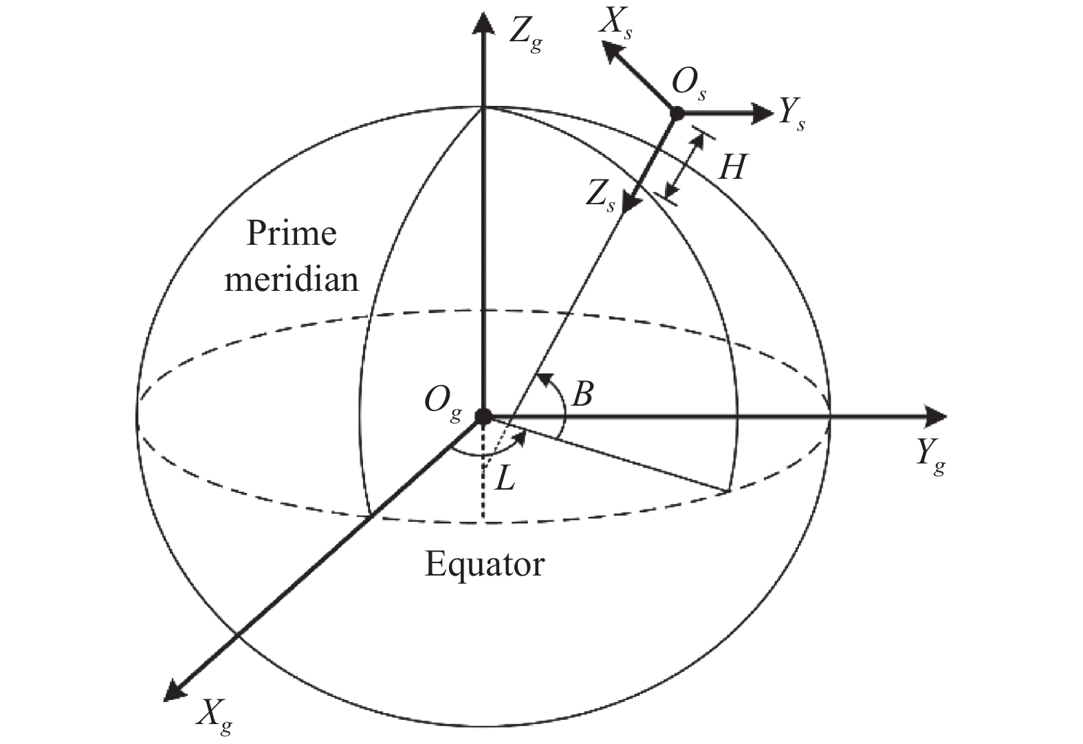
大地坐标系E以GPS采用的WGS-84基准建立,通过纬度B、经度L、高程H表示任意空间点位置。
-
地球空间直角坐标系G以WGS-84基本参数所定义的参考框架建立,原点处于地球中心,$ {Z}_{g} $轴与地球自转轴重合指向地理北极,$ {X}_{g} $轴从原点指向本初子午线与赤道的交点,$ {Y}_{g} $轴与$ {X}_{g} $轴和$ {Z}_{g} $轴构成右手坐标系,如图1所示,以($ {x}_{g},{y}_{g},{z}_{g} $)表示地球空间直角坐标系中任意一点位置。
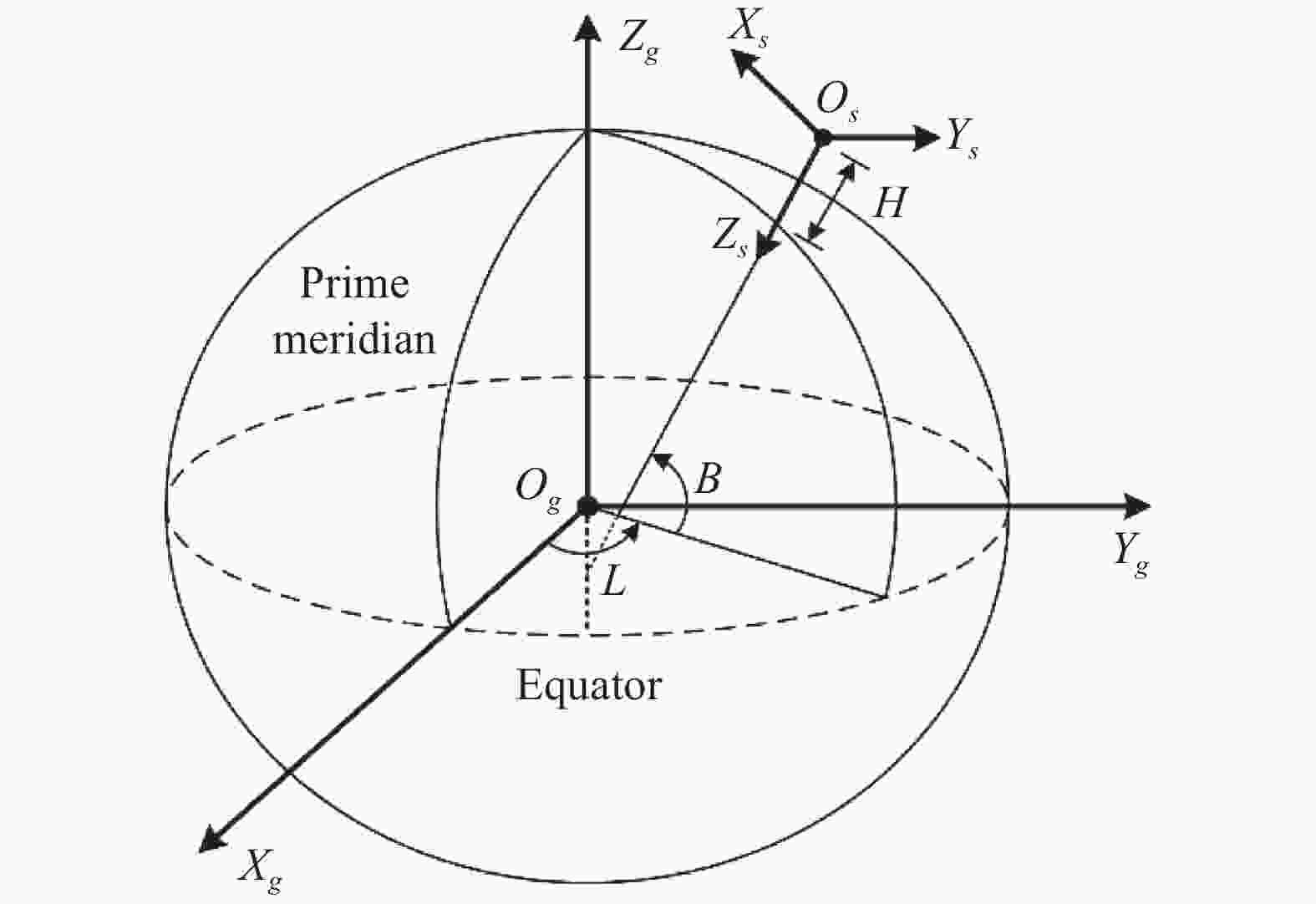
图 1 地球空间直角坐标系和载机地理坐标系
Figure 1. Geocentric coordinate system and aircraft geographic coordinate system
-
载机地理坐标系S原点即载机定位点,$ {X}_{s} $轴指向正北,$ {Y}_{s} $轴指向正东,$ {Z}_{s} $轴与$ {X}_{s} $轴和$ {Y}_{s} $轴形成右手坐标系垂直向下,即北东地坐标系(见图1),以($ {x}_{s},{y}_{s},{z}_{s} $)表示载机地理坐标系中任意一点位置。从S系到E系的转换过程见文献[5-13]。
-
机体坐标系A原点与载机地理坐标系原点一致,$ {X}_{a} $轴指向机头,$ {Y}_{a} $轴指向载机右侧,$ {Z}_{a} $轴垂直载机向下,三轴构成右手坐标系,即前右下坐标系,如图2所示,以($ {x}_{a},{y}_{a},{z}_{a} $)表示机体坐标系中任意一点位置。

图 2 机体坐标系
Figure 2. Aircraft coordinate system
从A系转换到S系的过程为:绕$ {Z}_{a} $轴旋转$ -{\psi }_{a} $,之后绕$ {Y}_{a} $轴旋转$ -{\theta }_{a} $,最后绕$ {X}_{a} $轴旋转$ -{\varphi }_{a} $,其中$ {\psi }_{a} $为载机偏航角,$ {\theta }_{a} $为载机俯仰角,$ {\varphi }_{a} $为载机横滚角,旋转矩阵为:
$$\begin{split} & {{{\boldsymbol{Q}}}}_{A}^{S}= {\boldsymbol{Q}} \left({\psi }_{a}\right){\boldsymbol{Q}} \left({\theta }_{a}\right){\boldsymbol{Q}}\left({\varphi }_{a}\right)=\\ & \left[\begin{array}{cccc}{C}_{{\psi }_{a}}{C}_{{\theta }_{a}}& {C}_{{\psi }_{a}}{S}_{{\theta }_{a}}{S}_{{\varphi }_{a}}-{S}_{{\psi }_{a}}{C}_{{\varphi }_{a}}& {C}_{{\psi }_{a}}{S}_{{\theta }_{a}}{C}_{{\varphi }_{a}}+{S}_{{\psi }_{a}}{S}_{{\varphi }_{a}}& 0\\ {S}_{{\psi }_{a}}{C}_{{\theta }_{a}}& {S}_{{\psi }_{a}}{S}_{{\theta }_{a}}{S}_{{\varphi }_{a}}+{C}_{{\psi }_{a}}{C}_{{\varphi }_{a}}& {S}_{{\psi }_{a}}{S}_{{\theta }_{a}}{C}_{{\varphi }_{a}}-{C}_{{\psi }_{a}}{S}_{{\varphi }_{a}}& 0\\ -{S}_{{\theta }_{a}}& {C}_{{\theta }_{a}}{S}_{{\varphi }_{a}}& {C}_{{\theta }_{a}}{C}_{{\varphi }_{a}}& 0\\ 0& 0& 0& 1\end{array}\right] \end{split}$$ (1) 式中:$ {C}_{{\psi }_{a}}=\cos{\psi }_{a} $;$ {S}_{{\psi }_{a}}=\sin{\psi }_{a} $。
-
光电吊舱通过减震器与载机连接,在不考虑机体振动引起减震器角振动误差情况下,认为吊舱基座坐标系与机体坐标系重合,以($ {x}_{b},{y}_{b},{z}_{b} $)表示吊舱基座坐标系中任意一点位置。当考虑减震器角震动误差时,坐标系转换过程和旋转矩阵与A系转换到S系类似。
-
相机坐标系C原点位于成像系统中心,$ {X}_{c} $轴与视轴方向一致指向目标点,当$ {X}_{c} $轴处于水平位置时,$ {Z}_{c} $轴指向垂直向下,$ {Y}_{c} $轴与$ {X}_{c} $轴和$ {Z}_{c} $轴构成右手坐标系,如图3所示,以($ {x}_{c},{y}_{c},{z}_{c} $)表示相机坐标系中任意一点位置。

图 3 相机坐标系
Figure 3. Camera coordinate system
从C系转换到B系的过程为:
绕$ {Z}_{c} $轴旋转$ -\alpha $,之后绕$ {Y}_{c} $轴旋转$ -\beta $,其中$ \alpha $为相机坐标系相对于吊舱基座坐标系的方位角,$\; \beta $为相机坐标系相对于吊舱基座坐标系的俯仰角,旋转矩阵为:
$$ \begin{array}{c}{\boldsymbol{Q}}_{C}^{B}={\boldsymbol{Q}}\left(\alpha \right){\boldsymbol{Q}}\left(\beta \right)=\left[\begin{array}{cccc}{C}_{\alpha }{C}_{\beta }& -{S}_{\alpha }& {C}_{\alpha }{S}_{\beta }& 0\\ {S}_{\alpha }{C}_{\beta }& {C}_{\alpha }& {S}_{\alpha }{S}_{\beta }& 0\\ -{S}_{\beta }& 0& {C}_{\beta }& 0\\ 0& 0& 0& 1\end{array}\right]\end{array} $$ (2) -
观测目标坐标系[14]T原点为观测目标位置点,$ {X}_{t} $轴、$ {Y}_{t} $轴和$ {Z}_{t} $轴分别与相机坐标系$ {X}_{c} $轴、$ {Y}_{c} $轴和$ {Z}_{c} $轴重合或平行,且方向一致,如图4所示,以($ {x}_{t},{y}_{t},{z}_{t} $)表示相机坐标系中任意一点位置。

图 4 观测目标坐标系
Figure 4. Observation target coordinate system
从T系转换到C系的过程为:
沿$ {X}_{t} $轴平移-R,R为目标点与成像系统的距离,平移矩阵为:
$$ \begin{array}{c}{\boldsymbol{Q}}_{T}^{C}=\left[\begin{array}{cccc}0& 0& 0& -R\\ 0& 0& 0& 0\\ 0& 0& 0& 0\\ 0& 0& 0& 1\end{array}\right]\end{array} $$ (3) -
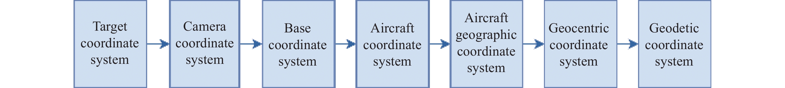
机载光电吊舱目标定位就是通过建立上述7个坐标系统,构建从观测目标坐标系到大地坐标系的定位模型,结合导航模块提供的载机位置和姿态信息、吊舱角度传感器提供的方位俯仰信息、激光测距机提供的距离信息,经过空间齐次坐标变换,得到目标大地坐标系位置。转换流程如图5所示。

图 5 坐标系转换流程
Figure 5. Process of coordinate system transformation
目标点在观测目标坐标系(T系)中的坐标为(0, 0, 0),结合各坐标系之间的变换公式,可得目标在大地坐标系(E系)中的经纬高坐标为($ {B}_{m},{L}_{m},{H}_{m} $),公式如下:
$$ \begin{array}{c}\left(\begin{array}{c}{B}_{m}\\ {L}_{m}\\ {H}_{m}\\ 1\end{array}\right)={\boldsymbol{Q}}_{G}^{E}{\boldsymbol{Q}}_{S}^{G}{\boldsymbol{Q}}_{A}^{S}{\boldsymbol{Q}}_{B}^{A}{\boldsymbol{Q}}_{C}^{B}{\boldsymbol{Q}}_{T}^{C}\left(\begin{array}{c}0\\ 0\\ 0\\ 1\end{array}\right)\end{array} $$ (4) -
文中旨在分析机载光电吊舱观瞄角度,因此需要构建观瞄角度测量模型。根据目标定位模型,可以推导出观瞄系统方位角和俯仰角的坐标转换过程,表示为:
$$ \begin{array}{c}\left(\begin{array}{c}\alpha \\ \beta \end{array}\right)={\boldsymbol{P}}\left(D\right)\end{array} $$ (5) 式中:$ \alpha $、$ \;\beta $为观瞄方位角和俯仰角;$ D $为转换过程中涉及的各项参数,具体包括:1)目标点大地坐标($ {B}_{m},{L}_{m},{H}_{m} $);2)载机大地坐标($ {B}_{a},{L}_{a},{H}_{a} $);3)载机姿态信息,偏航角、俯仰角、横滚角($ {\psi }_{a},{\theta }_{a},{\varphi }_{a} $);4)减震器振动误差,振动偏航角、振动俯仰角、振动横滚角($ \delta {\psi }_{b},\delta {\theta }_{b},\delta {\phi }_{b} $);$ \boldsymbol{P} $表示转换过程,由公式(4)推导得出。
-
观瞄角度计算过程所涉及参数产生的误差,会影响最终测角精度,根据上一节观瞄角度测量方程分析测量参数的误差来源主要包括:
1)目标点定位误差。若目标点位置信息是通过其他平台定位系统提供的测量值,则经度、纬度和高程信息会存在三个误差源$\delta {B}_{m}、\delta {L}_{m}、\delta {H}_{m}$;
2)载机定位误差。载机位置信息包含经度、纬度和高程,由机载导航系统提供,误差源表示为$\delta {B}_{a}、 \delta {L}_{a}、\delta {H}_{a}$;
3)载机姿态误差。载机姿态信息包含飞机偏航角、俯仰角、横滚角,由飞机惯性测量单元或组合导航模块提供,误差源表示为$\delta {\psi }_{a}、\delta {\theta }_{a}、\delta {\varphi }_{a}$;
4)减震器振动误差。光电吊舱基座与载机通过减震器连接,由于振动会产生三轴角误差,误差源表示为$\delta {\psi }_{b}、\delta {\theta }_{b}、\delta {\varphi }_{b}$;
5)目标指向误差。受到吊舱角度传感器精度、观瞄控制稳定精度等因素的影响,视轴对目标指向的误差源表示为$\delta \alpha 、\delta \beta$。目标指向误差可直观地描述观瞄轴的脱靶量。
上述测量参数误差源相互独立,通过观瞄角度测量方程进行传递,最终影响测角精度。设$\mathrm{\Delta }\alpha 、\mathrm{\Delta }\beta$为各误差源引起的观瞄角度方位、俯仰误差,$ {d}_{i} $为各参数真值,$ \delta {d}_{i} $为各参数误差,由观瞄角度测量方程(5)可得观瞄角度测量误差模型为:
$$\begin{split} \left(\begin{array}{c}\Delta \alpha \\ \Delta \beta \end{array}\right)= & {\boldsymbol{P}}\left({d}_{1}+\delta {d}_{1},{d}_{2}+\delta {d}_{2},\cdot \cdot \cdot ,{d}_{n}+\delta {d}_{n}\right)-\\ & {\boldsymbol{P}}\left({d}_{1},{d}_{2},\cdot \cdot \cdot ,{d}_{n}\right) \end{split} $$ (6) -
文中采用蒙特卡洛统计模拟方法,通过生成大量随机数据进行仿真,分析载机偏航角、载机俯仰角、载机横滚角、振动偏航角、振动俯仰角、振动横滚角、方位指向精度、俯仰指向精度8个测量参数对观瞄角度测量误差的影响。机载光电吊舱观瞄角度测量误差分析流程如下:
1)确定8个影响参数的误差源的随机分布形式及随机分布特征,见表1;
表 1 随机误差分布表
Table 1. Distributions of random errors
Error source Symbol Error distribution Standard deviation$ /{(}^{\circ }) $ Random error value Aircraft attitude $ \delta {\psi }_{a} $ Normal distribution $ {\sigma }_{{\psi }_{a}}=0.2 $ $ \delta {\psi }_{a}=\sigma {\psi }_{a}\cdot Randn\left( \right) $ $ \delta {\theta }_{a} $ Normal distribution $ {\sigma }_{{\theta }_{a}}=0.1 $ $ \delta {\theta }_{a}=\sigma {\theta }_{a}\cdot Randn\left( \right) $ $ \delta {\varphi }_{a} $ Normal distribution $ {\sigma }_{{\varphi }_{a}}=0.1 $ $ \delta {\varphi }_{a}=\sigma {\varphi }_{a}\cdot Randn\left( \right) $ Platform vibration isolator $ \delta {\psi }_{b} $ Normal distribution $ {\sigma }_{{\psi }_{b}}=0.1 $ $ \delta {\psi }_{b}=\sigma {\psi }_{b}\cdot Randn\left( \right) $ $ \delta {\theta }_{b} $ Normal distribution $ {\sigma }_{{\theta }_{b}}=0.1 $ $ \delta {\theta }_{b}=\sigma {\theta }_{b}\cdot Randn\left( \right) $ $ \delta {\varphi }_{b} $ Normal distribution $ {\sigma }_{{\varphi }_{b}}=0.1 $ $ \delta {\varphi }_{b}=\sigma {\varphi }_{b}\cdot Randn\left( \right) $ Target pointing $ \delta \alpha $ Uniform distribution $\delta {\alpha }_{\mathrm{m}\mathrm{a}\mathrm{x} }=0.001\;5$ $ \delta \alpha =2\delta {\alpha }_{\mathrm{m}\mathrm{a}\mathrm{x}}\left(Rand\left( \right)-0.5\right) $ $ \delta \beta $ Uniform distribution $\delta {\beta }_{\mathrm{m}\mathrm{a}\mathrm{x} }=0.001\;5$ $ \delta \beta =2\delta {\beta }_{\mathrm{m}\mathrm{a}\mathrm{x}}\left(Rand\left( \right)-0.5\right) $ 2)利用理论软件提供的随机数产生函数,生成若干组由服从各自误差分布的随机数组成的误差源随机向量;
3)设定一组初始值,首先根据公式(5)计算误差为零时的观瞄角度作为真值,然后将产生的误差源随机向量和真值代入公式(6),得到观瞄角度测量误差$\mathrm{\Delta }\alpha 、\mathrm{\Delta }\beta$;
4)对若干组观瞄角度测量误差进行统计,得到观瞄角总误差为:
$$ {\sigma }_{total}=\sqrt{\dfrac{1}{n}{\displaystyle\sum }_{i=1}^{n}\left(\mathrm{\Delta }{\alpha }_{i}^{2}+\mathrm{\Delta }{\beta }_{i}^{2}\right)}$$ (7) -
按照上节所述误差分析流程和表1数据进行$ 1{0}^{6} $次蒙特卡洛仿真实验,仿真结果如图6所示。对观瞄方位角误差和观瞄俯仰角误差结果分布进行统计,如图7所示。
图 6 观瞄角误差分布仿真图
Figure 6. Distribution of viewing angle error

图 7 (a) 观瞄方位角误差分布;(b) 观瞄俯仰角误差分布
Figure 7. (a) Distribution of viewing azimuth error; (b) Distribution of viewing pitch error
由误差统计结果可知,观瞄方位角误差和俯仰角误差分别服从标准差为$ {\sigma }_{\alpha }=0.225\;5 $和$ {\sigma }_{\beta }=0.141\;5 $的正态分布,观瞄角总误差$ {\sigma }_{total}=0.266\;248\;98 $。
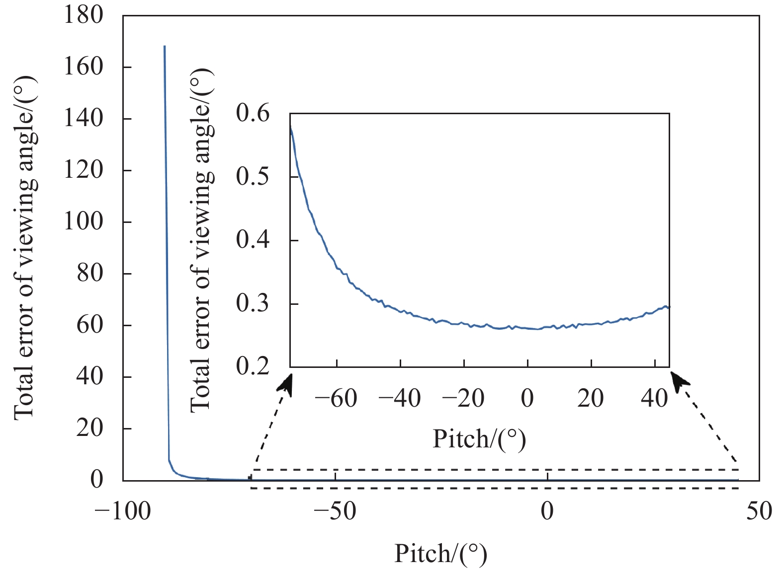
误差仿真过程中,在各误差源随机分布形式和随机分布特征一定的情况下,随着初始参数(目标及载机位置、载机姿态)设置的不同,出现了个别差异较大的仿真数据,为进一步分析仿真结果差异性的原因,设计仿真实验分析初始参数对观瞄角总误差影响。仿真结果表明,吊舱在S系中的俯仰角是引起观瞄角总误差突变的因素。仿真结果如图8所示。
图 8 俯仰角与观瞄角总误差的关系
Figure 8. Relation between pitch angle and total error of viewing angle
当吊舱在S系中的俯仰角从$ {0}^{\circ } $向$ -{90}^{\circ } $(负号表示转动方向)改变时,观瞄角总误差随着俯仰角增加呈指数增大的趋势,俯仰角从$ {0}^{\circ } $变化到$ -{40}^{\circ } $时,误差仅增大0.94%;从$ -{40}^{\circ } $变化到$ -{80}^{\circ } $时,误差增大19.43%。仿真数据表明,俯仰角转动量越接近$ {90}^{\circ } $,引起的观瞄角总误差越大,而小于$ {40}^{\circ } $时,俯仰角对观瞄角总误差的影响可以忽略。
为进一步分析各误差源对观瞄角总误差的影响,定义误差影响因子$ \tau $反映各误差源对观瞄角总误差的影响程度,具体定义如下:
$$ \begin{array}{c}{\tau }_{i}=\dfrac{{\sigma }_{total\_i}}{{\sigma }_{i}} \end{array} $$ (8) 式中:$ {\sigma }_{i} $为误差源$ i $的标准差;$ {\sigma }_{total\_i} $为仅施加误差源$ i $得到的观瞄角总误差。误差影响因子$ \tau $越大,则误差传递效率越高,误差源对观瞄角总误差影响程度越大。若$ \tau > 1 $则表明经过误差传递该误差被放大,若$ \tau < 1 $则表明经过误差传递该误差被缩小,若$ \tau =1 $则表明该误差等效传递至观瞄角总误差。分别计算各误差源单独作用时的观瞄角总误差$ {\sigma }_{total\_i} $,代入公式(8)得到误差影响因子$ {\tau }_{i} $,图9为载机姿态角误差影响因子随吊舱绝对俯仰角变化曲线。
图 9 俯仰角与载机姿态角误差影响因子的关系
Figure 9. Relation between pitch angle and error influence factor of aircraft attitude angle
载机偏航角误差影响因子在俯仰角趋于$ -{90}^{\circ } $时近似为0,其他位置近似为1;俯仰角误差影响因子和横滚角误差影响因子随俯仰角增加而增大,且越接近$ {90}^{\circ } $,误差影响因子变化越大,与观瞄角总误差变化趋势一致。振动误差规律与载机姿态角误差规律一致,目标指向误差影响因子不随俯仰角变化。可见载机姿态及振动的俯仰角误差和横滚角误差是影响观瞄角总误差随俯仰角增加呈指数增长的主要因素。
结合军事应用实际,在进行观瞄角引导时,无人机一般不会位于俯仰角较大的目标上方空域,俯仰角对观瞄角总误差的影响可以忽略。
表2为一组误差源影响因子,可以看出,载机偏航角、俯仰角、横滚角误差分别和减震器偏航振动、俯仰振动、横滚振动误差影响因子趋于一致,目标指向方位误差和目标指向俯仰误差的影响因子近似相等,能够与构建的测量模型对应。其中,载机偏航角误差和振动偏航角误差的传递效率近似为100%,载机俯仰角误差和振动俯仰角误差的传递效率约为94%,目标指向误差传递效率约为57%,载机横滚角误差和振动横滚角误差的传递效率仅约34%。因此,在进行观瞄角引导时,载机偏航角和振动偏航角误差影响最大,载机横滚角和振动横滚角误差影响最小。
表 2 误差影响因子
Table 2. Error influence factor
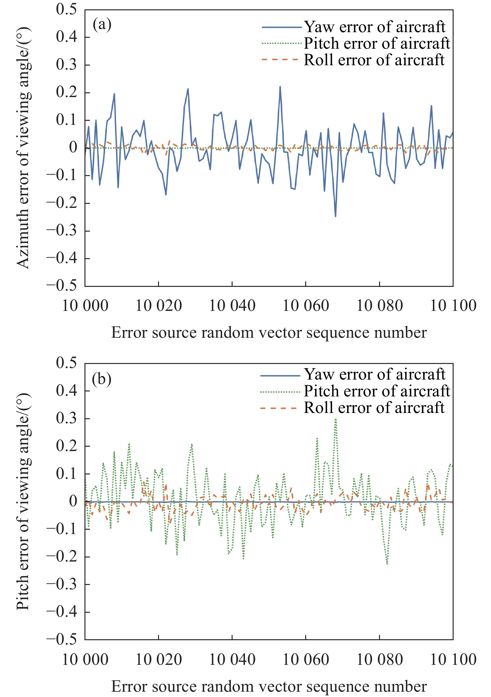
Error source $ {\sigma }_{total\_i}/{(}^{\circ }) $ $ {\tau }_{i} $ $ \delta {\psi }_{a} $ 0.2012 1.0061 $ \delta {\theta }_{a} $ 0.0943 0.9430 $ \delta {\varphi }_{a} $ 0.0344 0.3440 $ \delta {\psi }_{b} $ 0.1002 1.0019 $ \delta {\theta }_{b} $ 0.0946 0.9465 $ \delta {\varphi }_{b} $ 0.0345 0.3445 $ \delta \alpha $ $8.665\;1\times {10}^{-4}$ 0.5777 $ \delta \beta $ $8.664\;3\times {10}^{-4}$ 0.5776 为了能够更加直观的对比载机各姿态角误差对观瞄角误差的影响程度,对仿真数据进行处理,生成观瞄方位角和俯仰角误差曲线,图10选取了其中区间长度为100的误差曲线。
可明显看出载机偏航角误差对观瞄方位角影响较大,载机俯仰角误差对观瞄方位角影响很小,同样,姿态角误差中对观瞄俯仰角影响最大的是载机俯仰角误差,而载机偏航角误差的影响与之相比微乎其微。减震器振动误差的影响情况与之类似。
图 10 (a) 载机姿态角误差对观瞄方位角误差的影响;(b) 载机姿态角误差对观瞄俯仰角误差的影响
Figure 10. (a) Effect of aircraft attitude angle error on viewing azimuth error; (b) Effect of aircraft attitude angle error on viewing pitch error
-
误差分析模型是通过各单项测量误差的分布形式及分布特征推导其对总误差的影响,而在系统总体设计时,通常依据总体精度要求对误差传递过程中各参数指标进行分配,再通过大量的仿真实验对各项误差进行标校调整,使得最终误差分配结果既满足总体精度要求,又能够在工程上实现。传统的误差分配方法包括平均分配法和加权分配法,文中提出采用改进麻雀优化算法(ISSA)进行误差分配。
-
平均分配法按照等作用原则对误差进行分配,假设各误差源对总误差的影响相同,则各误差源标准差为:
$$ \begin{array}{c}{\sigma }_{mean\_i}=\dfrac{{\sigma }_{total}}{n}={\sigma }_{i}\left(i=\mathrm{1,2},\cdot \cdot \cdot ,n\right)\end{array} $$ (9) 式中:$ {\sigma }_{mean\_i} $为平均分配法得到的各误差源标准差;$ {\sigma }_{total} $为待分配总误差;n为误差源个数。将由表1得到的观瞄角总误差$ {\sigma }_{total}=0.266\;248\;98 $代入公式(9),得到一组$ {\sigma }_{mean\_i}={0.033\;281\;12} $的误差分配方案,进行蒙特卡洛仿真实验,此时观瞄角总误差$ {\sigma }_{total\_mean}= {0.072\;134\;04} $。
平均分配法简单易行,但是这种分配方法假定各误差源对总误差的影响完全相同,各误差源分配结果相同,满足其中一些误差源的精度要求较为容易,而满足另一些误差源精度要求则颇为困难,需要用昂贵的高精度仪器。
-
加权分配法按照一定的权重对误差进行分配,文中根据表2的误差影响因子确定误差分配权重,则各误差源标准差为:
$$ \begin{array}{c}{\sigma }_{weight\_i}=\dfrac{{\tau }_{i}}{{\displaystyle\sum }_{i=1}^{n}{\tau }_{i}}{\sigma }_{total}\left(i=\mathrm{1,2},\cdot \cdot \cdot ,n\right)\end{array} $$ (10) 式中:$ {\sigma }_{weight\_i} $为加权分配法得到的各误差源标准差;$ {\tau }_{i} $为表2中误差影响因子。由$ {\sigma }_{weight\_i} $构成的误差分配方案及该方案观瞄角总误差$ {\sigma }_{total\_weight} $见表3。
表 3 加权分配法误差分配结果
Table 3. Error distribution results of weighted distribution method
Error source Weight coefficient Standard deviation$ /{(}^{\circ }) $ $ \delta {\psi }_{a} $ 0.1753 $ {\sigma }_{weight\_{\psi }_{a}}=\text{0.046\;7} $ $ \delta {\theta }_{a} $ 0.1642 $ {\sigma }_{weight\_{\theta }_{a}}=\text{0.043\;7} $ $ \delta {\varphi }_{a} $ 0.0599 $ {\sigma }_{weight\_{\varphi }_{a}}=\text{0.016\;0} $ $ \delta {\psi }_{b} $ 0.1753 $ {\sigma }_{weight\_{\psi }_{b}}=\text{0.046\;7} $ $ \delta {\theta }_{b} $ 0.1642 $ {\sigma }_{weight\_{\theta }_{b}}=\text{0.043\;7} $ $ \delta {\varphi }_{b} $ 0.0599 $ {\sigma }_{weight\_{\varphi }_{b}}=\text{0.016\;0} $ $ \delta \alpha $ 0.1006 $ \delta {\alpha }_{weight\_\mathrm{m}\mathrm{a}\mathrm{x}}=\text{0.026\;8} $ $ \delta \beta $ 0.1006 $ \delta {\beta }_{weight\_\mathrm{m}\mathrm{a}\mathrm{x}}=\text{0.026\;8} $ $ {\sigma }_{total\_weight} $ 0.09133344 加权分配法考虑了各测量值的重要性和精确度,增加对总误差影响较大的误差源分配比例,减少对总误差影响较小的误差源分配比例,使分配结果更加合理,但是在工程实际中通过加权分配法确定各误差源权重往往非常复杂,通常要结合从业者的主观判断和经验积累。
-
每组分配方案对应一组误差源标准差,若将每组误差源标准差作为变量进行优化,使得最优变量造成的观瞄角总误差无限逼近待分配指标,则可将误差分配问题转化为参数优化问题并通过优化算法解决。
-
麻雀算法(SSA)是在模仿麻雀觅食和逃避捕食者的行为基础上,增加危险预警机制而提出的群智能优化算法[15],该算法局部搜索能力极强,收敛速度较快。然而在对文中误差分配问题的优化精度方面,SSA算法与遗传算法(GA)和粒子群算法(PSO)相比不具备优势,进而融合单纯形算法对基本SSA算法进行改进,采用改进麻雀优化算法(ISSA)对机载光电吊舱观瞄角度误差分配进行优化。
1)目标函数的构建。
由公式(6)和公式(7)可以得到误差源分配方案$ {X}_{i} $及其导致的观瞄角总误差$ {\sigma }_{total\_i} $与待分配指标差值的映射关系为:
$$ \begin{array}{c}\Delta \varepsilon =f\left({X}_{i}\right)={\sigma }_{total}-{\sigma }_{tota{l}_{i}}\end{array} $$ (11) 式中:$ {\Delta }\varepsilon $为误差分配余量,该值越小则表明误差分配效果越好。若仅考虑差值最小,则$ f\left({X}_{i}\right) $即为目标函数,然而在实际误差分配过程中,必须考虑误差源分配方案$ {X}_{i} $导致的观瞄角总误差不得超过待分配指标,即在进行优化时,需使$ {\Delta }\varepsilon \to {0}^{+} $,若$ {\Delta }\varepsilon < 0 $,则需要构造惩罚函数进行约束,因此目标函数可表示为:
$$ \begin{array}{c}T\left({X}_{i}\right)=f\left({X}_{i}\right)+{\min}\left({{\rm{sgn}}}\left({\Delta }\varepsilon \right),0\right)\end{array} $$ (12) 2)采用单纯形算法二次优化。
为了克服SSA算法局部最优的问题,在SSA算法麻雀位置(误差源分配方案)更新后,根据适应度进行排序,利用单纯形算法对适应度最优和最差的各10%麻雀位置进行二次优化。
单纯形算法基于几何学中单纯形的概念,通过构造一个N+1维的单纯形,计算比较各顶点的目标函数值,并以目标函数值较小的顶点取代目标函数值最大的顶点来构建新的单纯形,迭代循环直至达到收敛条件[16]。
单纯形算法搜索最小值的基本原理如下:
1)初始化:初始化N+1个点$ {X}_{1},{X}_{2},\cdot \cdot \cdot ,{X}_{N},{X}_{N+1} $作为N+1维单纯形的顶点,一个误差源分配方案即为单纯形的一个顶点;
2)排序:根据目标函数值$ T\left({X}_{i}\right) $对顶点进行排序,$ T\left({X}_{1}\right)\leqslant T\left({X}_{2}\right)\leqslant \cdot \cdot \cdot \leqslant T\left({X}_{N}\right)\leqslant T\left({X}_{N+1}\right) $;
3)计算质心位置:去除目标函数值最差的顶点$ {X}_{N+1} $,计算前N个点的质心$ {X}_{0}=\dfrac{1}{N}{\displaystyle\sum }_{i=1}^{N}{X}_{i} $;
4)计算反射点位置:对最差点$ {X}_{N+1} $进行反射操作,取$ {X}_{r}={X}_{0}+\rho \left({X}_{0}-{X}_{N+1}\right) $,$ {X}_{r} $是$ {X}_{N+1} $关于$ {X}_{0} $的反射点,其中$\; \rho $为反射系数,通常取$\; \rho =1 $;
5)判别搜索策略:
①计算反射点位置:对最差点$ {X}_{N+1} $进行反射操作,取$ {X}_{r}={X}_{0}+\;\rho \left({X}_{0}-{X}_{N+1}\right) $,$ {X}_{r} $是$ {X}_{N+1} $关于$ {X}_{0} $的反射点,其中$ \;\rho $为反射系数,通常取$ \;\rho =1 $;
②若$ T\left({X}_{1}\right) \leqslant T\left({X}_{r}\right) \leqslant T\left({X}_{N}\right) $,表明搜索方向正确,但无需进行扩张操作,令$ {X}_{N+1}={X}_{r} $;
③若$ T\left({X}_{N}\right) < T\left({X}_{r}\right) < T\left({X}_{N+1}\right) $,表明搜索方向正确,但搜索距离过大,需进行收缩操作,取$ {X}_{c}={X}_{0}+ \kappa \left({X}_{r}-{X}_{0}\right) $,$ \kappa $为收缩系数,通常取$ \kappa =0.5 $;如果$ T\left({X}_{c}\right)\leqslant T\left({X}_{N+1}\right) $,则令$ {X}_{N+1}={X}_{c} $,反之则令所有点向最优点收缩,即$ {X}_{i}={X}_{1}+\nu \left({X}_{i}-{X}_{1}\right) $,$ \nu $为回退系数,通常取$ \nu =0.5 $;
④若$ T\left({X}_{N+1}\right) \leqslant T\left({X}_{r}\right) $,表明搜索方向错误,需要进行内缩操作,取$ {X}_{s}={X}_{0}-\kappa \left({X}_{0}-{X}_{N+1}\right) $,如果$ T\left({X}_{s}\right) < T\left({X}_{N+1}\right) $,则令$ {X}_{N+1}={X}_{s} $,反之则令所有点向最优点收缩,即$ {X}_{i}={X}_{1}+\nu \left({X}_{i}-{X}_{1}\right) $;
6)检查结束条件:如满足结束条件,则输出各顶点(误差源分配方案),反之转入第2)步骤,继续执行。
-
仿真优化效果见图11,与SSA算法、GA算法和PSO算法进行对比实验[17-18],文中采用的ISSA算法在解决机载光电吊舱观瞄角度误差分配问题上具有一定优势,能够克服SSA算法陷入局部极值的问题,具有良好的全局搜索能力,与GA和PSO算法相比,收敛速度快,优化效果好。误差分配结果见表4。

图 11 算法优化效果对比图
Figure 11. Comparison of algorithm optimization effect
表 4 基于ISSA算法的误差分配结果
Table 4. Error allocation results based on ISSA
Error source Standard error$ /{(}^{\circ }) $ $ \delta {\psi }_{a} $ $ {\sigma }_{IS S A\_{\psi }_{a}}=\text{0.148\;2} $ $ \delta {\theta }_{a} $ $ {\sigma }_{IS S A\_{\theta }_{a}}=\text{0.031\;2} $ $ \delta {\varphi }_{a} $ $ {\sigma }_{IS S A\_{\varphi }_{a}}=\text{0.125\;6} $ $ \delta {\psi }_{b} $ $ {\sigma }_{IS S A\_{\psi }_{b}}=\text{0.027\;3} $ $ \delta {\theta }_{b} $ $ {\sigma }_{IS S A\_{\theta }_{b}}=\text{0.171\;1} $ $ \delta {\varphi }_{b} $ ${\sigma }_{IS S A\_{\varphi }_{b} }=\text{0.046\;5}$ $ \delta \alpha $ $ \delta {\alpha }_{IS S A\_\mathrm{m}\mathrm{a}\mathrm{x}}=\text{0.195\;1} $ $ \delta \beta $ $ \delta {\beta }_{IS S A\_\mathrm{m}\mathrm{a}\mathrm{x}}=\text{0.064\;8} $ $ {\sigma }_{total\_IS S A} $ 0.26624896 将平均分配法、加权分配法以及改进麻雀算法给出的误差分配方案导致的观瞄角总误差以及误差分配余量进行汇总,如表5所示。
通过对比数据可知,采用平均分配法和加权分配法得到的误差分配结果都能满足待分配总误差的要求,相较而言,加权分配法使总误差更接近于待分配指标,但是两种方法的分配结果均未达到各误差源允许误差的极限值,还需进行反复试凑,在工程实践中,权重确定通常依赖经验数据,具有很大的局限性。采用基于ISSA分配法得到的最优分配方案非常接近待分配总误差,使待分配误差得到充分利用,在解决误差参数多、误差传递过程复杂的问题上优势明显,显著提升了误差分配的效率,但是此方法是在数值上追求误差分配余量最小,若想得到理想的分配方案,还需设定各误差源参数优化范围,然而相较于加权法权重的确定,误差源范围的设置更为客观、便捷。
表 5 各分配方法效果对比
Table 5. Distribution method effect comparison
Distribution method Total error of viewing angle$ /{(}^{\circ }) $ Margin of error distribution$ /{(}^{\circ }) $ Equal distribution $ {\sigma }_{total\_mean}=\text{0.072\;134\;04} $ 0.1941 Weighted distribution $ {\sigma }_{total\_weight}=0.091\;333\;44 $ 0.1749 ISSA algorithm distribution ${\sigma }_{total\_IS S A}=0.266\;248\;96$ 2.3347×10⁻⁸ -
文中结合小微型无人机载光电吊舱特点,利用空间齐次坐标变换法分析定位及引导过程,通过建立7个坐标系,构建观瞄角测量模型和误差模型。采用蒙特卡洛模拟方法进行误差分析,以误差影响因子量化各误差源对总误差的影响程度,模拟仿真实验结果表明,载机偏航角和振动偏航角误差对观瞄角总误差影响最大,误差传递效率近似为100%,载机横滚角和振动横滚角误差对观瞄角总误差影响最小,传递效率仅约34%。采用基于单纯形的麻雀优化算法进行误差分配,将误差分配问题转化为参数优化问题进行处理,与平均分配法和加权分配法相比,充分发挥了各误差源的最大允许误差,误差分配余量能够达到$ 1{0}^{-8} $量级,避免了反复试凑,更加便捷高效;与遗传算法和粒子群算法相比,文中采用的改进麻雀优化算法收敛速度更快,优化效果更好。
文中通过仿真实验定量分析了观瞄角引导误差与各误差源之间的关系,并验证了基于单纯形的麻雀优化算法进行误差分配的可行性。然而基于优化算法的误差分配方法是一种数据上的拟合,在指导实际工程应用时,如果能够结合误差分配侧重点、各参数测量单元当前技术发展水平以及制造成本等多方面因素,设定参数优化范围,确定最理想的误差分配方案,并以该方案指导关键器件的选型,将会更具有指导意义,这也是文中后续的研究方向。
Research on the error distribution method of unmanned airborne electro-optical pod viewing angle
-
摘要: 针对无人机载光电吊舱总体设计过程中高效便捷地分配各测量模块的误差,以便确定最优器材选型方案的需求,提出了一种基于单纯形策略的改进麻雀算法,从多目标优化角度对小微型无人机载光电吊舱观瞄角误差分配问题进行研究。首先根据小微型无人机载光电吊舱的特点建立坐标系,利用空间齐次坐标变换法推导目标定位及观瞄角测量模型;然后分析误差主要来源,建立观瞄角误差模型,基于蒙特卡洛模拟法进行误差分析;最后以观瞄角误差模型为基础,采用平均分配法、加权分配法以及改进麻雀算法进行误差分配,并对分配结果进行对比分析。仿真实验结果表明,载机偏航角误差和振动偏航角误差对观瞄角总误差影响最大,误差传递效率近似为100%,载机横滚角误差和振动横滚角误差对观瞄角总误差影响最小,误差传递效率仅约34%;改进麻雀算法的误差分配余量能够达到$ 1{0}^{-8} $量级,与传统误差分配方法相比显著提高了分配效率,验证了基于单纯形策略的改进麻雀算法解决小微型无人机载光电吊舱观瞄角误差分配问题的有效性。Abstract:
Objective The airborne electro-optical pods require high accuracy in viewing angle orientation when performing tasks such as autonomous target localization and simulating counter targets. Medium and large military airborne electro-optical pods often use high-performance measurement units, such as integrated sub-inertial guidance systems, to avoid the effects of errors caused by vibration to improve guidance accuracy. However, due to the limitation of size, weight, and power of the small and micro-unmanned airborne optoelectronic pods, their related measurement modules for viewing angle orientation are degraded in performance, and the viewing angle orientation accuracy is bound to decrease. In addition, the cost-effectiveness ratio is also an essential factor of modern unmanned combat. Therefore, how to select cost-effective components while ensuring overall accuracy is the primary problem when conducting the overall design of small and micro-unmanned airborne electro-optical pods. For this reason, an improved sparrow algorithm based on the simplex strategy is proposed in this paper to study the error distribution problem of small and micro-unmanned airborne electro-optical pod viewing angle from the perspective of multi-objective optimization, which provides a basis for engineering design and equipment selection. Methods Firstly, the coordinate system is established according to the characteristics of the small and micro UAV photoelectric pod, and the viewing angle measurement model is derived by using the spatial homogeneous coordinate transformation method; Then the principal sources of errors are analyzed, the viewing angle error model is established, and error analysis is performed based on Monte Carlo simulation method; Finally, based on the viewing angle error model, the improved sparrow algorithm based on the simplex strategy proposed in this paper is used for error distribution, and compared with the average distribution method, the weighted distribution method, and the error distribution methods based on genetic algorithm and particle swarm algorithm. Results and Discussions The improved sparrow algorithm based on simplex strategy proposed in this paper has certain advantages in solving the error allocation problem with multiple error parameters and complex error transmission process. Compared with the sparrow algorithm, genetic algorithm, and particle swarm algorithm, the improved algorithm has faster convergence and better optimization effect, overcomes the problem that the sparrow algorithm falls into local extremes, and has good global search ability (Fig.11). Compared with the traditional error distribution method, the error distribution margin of the optimal distribution scheme obtained by the improved algorithm can reach the magnitude of $ 1{0}^{-8} $(Tab.5), which significantly improves the efficiency of the error distribution. Conclusions In this paper, Monte Carlo simulation method is used to analyze the error of the viewing angle of the electro-optical pod, and an improved sparrow algorithm based on the simplex strategy is proposed for error distribution. The simulation results of error analysis show that the carrier yaw angle error and vibration yaw angle error have the greatest impact on the total error of the viewing angle, and the error transfer efficiency is slightly more than 100%, while the carrier roll angle error and vibration roll angle error have the least impact on the total error of the viewing angle, and the error transfer efficiency is only about 34%; The simulation results of error distribution show that the error distribution margin of the improved sparrow algorithm can reach the magnitude of 10-8, which significantly improves the distribution efficiency compared with the traditional error distribution method, and verifies the effectiveness of the improved sparrow algorithm based on the simplex strategy to solve the error distribution problem of the viewing angle of the electro-optical pod. However, the error distribution method based on the optimization algorithm is a kind of data fitting. When guiding practical engineering applications, it will be more instructive if the optimization range can be set with the design focus to determine the optimal error allocation scheme and use this scheme to guide the selection of crucial devices, which is also the subsequent research direction of this paper. -
图 1 地球空间直角坐标系和载机地理坐标系
Figure 1. Geocentric coordinate system and aircraft geographic coordinate system
图 7 (a) 观瞄方位角误差分布;(b) 观瞄俯仰角误差分布
Figure 7. (a) Distribution of viewing azimuth error; (b) Distribution of viewing pitch error
图 8 俯仰角与观瞄角总误差的关系
Figure 8. Relation between pitch angle and total error of viewing angle
图 9 俯仰角与载机姿态角误差影响因子的关系
Figure 9. Relation between pitch angle and error influence factor of aircraft attitude angle
图 10 (a) 载机姿态角误差对观瞄方位角误差的影响;(b) 载机姿态角误差对观瞄俯仰角误差的影响
Figure 10. (a) Effect of aircraft attitude angle error on viewing azimuth error; (b) Effect of aircraft attitude angle error on viewing pitch error
表 1 随机误差分布表
Table 1. Distributions of random errors
Error source Symbol Error distribution Standard deviation$ /{(}^{\circ }) $ Random error value Aircraft attitude $ \delta {\psi }_{a} $ Normal distribution $ {\sigma }_{{\psi }_{a}}=0.2 $ $ \delta {\psi }_{a}=\sigma {\psi }_{a}\cdot Randn\left( \right) $ $ \delta {\theta }_{a} $ Normal distribution $ {\sigma }_{{\theta }_{a}}=0.1 $ $ \delta {\theta }_{a}=\sigma {\theta }_{a}\cdot Randn\left( \right) $ $ \delta {\varphi }_{a} $ Normal distribution $ {\sigma }_{{\varphi }_{a}}=0.1 $ $ \delta {\varphi }_{a}=\sigma {\varphi }_{a}\cdot Randn\left( \right) $ Platform vibration isolator $ \delta {\psi }_{b} $ Normal distribution $ {\sigma }_{{\psi }_{b}}=0.1 $ $ \delta {\psi }_{b}=\sigma {\psi }_{b}\cdot Randn\left( \right) $ $ \delta {\theta }_{b} $ Normal distribution $ {\sigma }_{{\theta }_{b}}=0.1 $ $ \delta {\theta }_{b}=\sigma {\theta }_{b}\cdot Randn\left( \right) $ $ \delta {\varphi }_{b} $ Normal distribution $ {\sigma }_{{\varphi }_{b}}=0.1 $ $ \delta {\varphi }_{b}=\sigma {\varphi }_{b}\cdot Randn\left( \right) $ Target pointing $ \delta \alpha $ Uniform distribution $\delta {\alpha }_{\mathrm{m}\mathrm{a}\mathrm{x} }=0.001\;5$ $ \delta \alpha =2\delta {\alpha }_{\mathrm{m}\mathrm{a}\mathrm{x}}\left(Rand\left( \right)-0.5\right) $ $ \delta \beta $ Uniform distribution $\delta {\beta }_{\mathrm{m}\mathrm{a}\mathrm{x} }=0.001\;5$ $ \delta \beta =2\delta {\beta }_{\mathrm{m}\mathrm{a}\mathrm{x}}\left(Rand\left( \right)-0.5\right) $  下载: 导出CSV
表 2 误差影响因子
Table 2. Error influence factor
Error source $ {\sigma }_{total\_i}/{(}^{\circ }) $ $ {\tau }_{i} $ $ \delta {\psi }_{a} $ 0.2012 1.0061 $ \delta {\theta }_{a} $ 0.0943 0.9430 $ \delta {\varphi }_{a} $ 0.0344 0.3440 $ \delta {\psi }_{b} $ 0.1002 1.0019 $ \delta {\theta }_{b} $ 0.0946 0.9465 $ \delta {\varphi }_{b} $ 0.0345 0.3445 $ \delta \alpha $ $8.665\;1\times {10}^{-4}$ 0.5777 $ \delta \beta $ $8.664\;3\times {10}^{-4}$ 0.5776
下载: 导出CSV
表 3 加权分配法误差分配结果
Table 3. Error distribution results of weighted distribution method
Error source Weight coefficient Standard deviation$ /{(}^{\circ }) $ $ \delta {\psi }_{a} $ 0.1753 $ {\sigma }_{weight\_{\psi }_{a}}=\text{0.046\;7} $ $ \delta {\theta }_{a} $ 0.1642 $ {\sigma }_{weight\_{\theta }_{a}}=\text{0.043\;7} $ $ \delta {\varphi }_{a} $ 0.0599 $ {\sigma }_{weight\_{\varphi }_{a}}=\text{0.016\;0} $ $ \delta {\psi }_{b} $ 0.1753 $ {\sigma }_{weight\_{\psi }_{b}}=\text{0.046\;7} $ $ \delta {\theta }_{b} $ 0.1642 $ {\sigma }_{weight\_{\theta }_{b}}=\text{0.043\;7} $ $ \delta {\varphi }_{b} $ 0.0599 $ {\sigma }_{weight\_{\varphi }_{b}}=\text{0.016\;0} $ $ \delta \alpha $ 0.1006 $ \delta {\alpha }_{weight\_\mathrm{m}\mathrm{a}\mathrm{x}}=\text{0.026\;8} $ $ \delta \beta $ 0.1006 $ \delta {\beta }_{weight\_\mathrm{m}\mathrm{a}\mathrm{x}}=\text{0.026\;8} $ $ {\sigma }_{total\_weight} $ 0.09133344
下载: 导出CSV
表 4 基于ISSA算法的误差分配结果
Table 4. Error allocation results based on ISSA
Error source Standard error$ /{(}^{\circ }) $ $ \delta {\psi }_{a} $ $ {\sigma }_{IS S A\_{\psi }_{a}}=\text{0.148\;2} $ $ \delta {\theta }_{a} $ $ {\sigma }_{IS S A\_{\theta }_{a}}=\text{0.031\;2} $ $ \delta {\varphi }_{a} $ $ {\sigma }_{IS S A\_{\varphi }_{a}}=\text{0.125\;6} $ $ \delta {\psi }_{b} $ $ {\sigma }_{IS S A\_{\psi }_{b}}=\text{0.027\;3} $ $ \delta {\theta }_{b} $ $ {\sigma }_{IS S A\_{\theta }_{b}}=\text{0.171\;1} $ $ \delta {\varphi }_{b} $ ${\sigma }_{IS S A\_{\varphi }_{b} }=\text{0.046\;5}$ $ \delta \alpha $ $ \delta {\alpha }_{IS S A\_\mathrm{m}\mathrm{a}\mathrm{x}}=\text{0.195\;1} $ $ \delta \beta $ $ \delta {\beta }_{IS S A\_\mathrm{m}\mathrm{a}\mathrm{x}}=\text{0.064\;8} $ $ {\sigma }_{total\_IS S A} $ 0.26624896
下载: 导出CSV
表 5 各分配方法效果对比
Table 5. Distribution method effect comparison
Distribution method Total error of viewing angle$ /{(}^{\circ }) $ Margin of error distribution$ /{(}^{\circ }) $ Equal distribution $ {\sigma }_{total\_mean}=\text{0.072\;134\;04} $ 0.1941 Weighted distribution $ {\sigma }_{total\_weight}=0.091\;333\;44 $ 0.1749 ISSA algorithm distribution ${\sigma }_{total\_IS S A}=0.266\;248\;96$ 2.3347×10⁻⁸
下载: 导出CSV
-
[1] 吉书鹏. 机载光电载荷装备发展与关键技术[J]. 航空兵器, 2017(06): 3-12. doi: 10.19297/j.cnki.41-1228/tj.2017.06.001 Ji Shupeng. Equipment development of airborne electro-optic payload and its key technologies [J]. Aero Weaponry, 2017(6): 3-12. (in Chinese) doi: 10.19297/j.cnki.41-1228/tj.2017.06.001 [2] 张帅, 韩松伟, 白冠冰, 等. 基于基准点引导的无人机光电平台定位精度分析与研究[J]. 电子技术与软件工程, 2021(24): 214-219. [3] 陈丹琪, 金国栋, 谭立宁, 等. 无人机载光电平台目标定位方法综述[J]. 飞航导弹, 2019(8): 43-48. doi: 10.16338/j.issn.1009-1319.20190063 [4] 钟麟, 张岐坦. 基于无人机载光电平台的目标定位技术[J]. 计算机与网络, 2021, 47(13): 53-57. doi: 10.3969/j.issn.1008-1739.2021.13.047 Zhong Lin, Zhang Qitan. Target localization technology of UAV photoelectric platform [J]. Computer & Network, 2021, 47(13): 53-57. (in Chinese) doi: 10.3969/j.issn.1008-1739.2021.13.047 [5] 王家骐, 金光, 颜昌翔. 机载光电跟踪测量设备的目标定位误差分析[J]. 光学精密工程, 2005(02): 105-116. doi: 10.3321/j.issn:1004-924X.2005.02.001 Wang Jiaqi, Jin Guang, Yan Changxiang. Orientation error analysis of airborne opto-electric tracking and measuring device [J]. Optics and Precision Engineering, 2005,13(2): 105-116. (in Chinese) doi: 10.3321/j.issn:1004-924X.2005.02.001 [6] 王晶, 高利民, 姚俊峰. 机载测量平台中的坐标转换误差分析[J]. 光学精密工程, 2009, 17(02): 388-94. doi: 10.3321/j.issn:1004-924X.2009.02.024 Wang Jing, Gao Limin, Yao Junfeng. Analysis on coordinate conversion error of airborne measuring device [J]. Optics and Precision Engineering, 2009, 17(2): 388-394. (in Chinese) doi: 10.3321/j.issn:1004-924X.2009.02.024 [7] 王增发, 孙丽娜, 李刚, 等. 机载光电平台自主引导精度分析[J]. 红外与激光工程, 2014, 43(11): 3585-91. doi: 10.3969/j.issn.1007-2276.2014.11.014 Wang Zengfa, Sun Lina, Li Gangzhang, et al. Accuracy analysis on autonomous guiding of airborne opto-electronic platform [J]. Infrared and Laser Engineering, 2014, 43(11): 3585-91. (in Chinese) doi: 10.3969/j.issn.1007-2276.2014.11.014 [8] 黄小帅, 王增发. 光电有源定位法精度分析及提升方法研究[J]. 电子技术与软件工程, 2021(8): 109-114. [9] 孙辉. 机载光电平台目标定位与误差分析[J]. 中国光学, 2013, 6(06): 912-8. Sun Hui. Target localization and error analysis of airborne electro-optical platform [J]. Chinese Optics, 2013, 6(6): 912-8. (in Chinese) [10] 徐诚, 黄大庆. 无人机光电侦测平台目标定位误差分析[J]. 仪器仪表学报, 2013, 34(10): 2265-70. doi: 10.19650/j.cnki.cjsi.2013.10.016 Xu Cheng, Huang Daqing. Error analysis for target localization with unmanned aerial vehicle electro-optical detection platform [J]. Chinese Journal of Scientific Instrument, 2013, 34(10): 2265-70. (in Chinese) doi: 10.19650/j.cnki.cjsi.2013.10.016 [11] 管坐辇, 王乃祥, 徐宁. 基于蒙特卡洛模拟的机载光电平台测角精度分析[J]. 电子测量与仪器学报, 2015, 29(03): 447-53. doi: 10.13382/j.jemi.2015.03.018 Guan Zuonian, Wang Naixiang, Xu Ning. Analysis of angle accuracy of airborne photoelectric platform based on Monte Carlo simulation [J]. Journal of Electronic Measurement and Instrumentation, 2015, 29(3): 447-453. (in Chinese) doi: 10.13382/j.jemi.2015.03.018 [12] 陈水忠, 王凯. 基于鱼群算法的机载光电平台误差分配方法[J]. 激光与红外, 2017, 47(05): 600-5. doi: 10.3969/j.issn.1001-5078.2017.05.015 Chen Shuizhong, Wang Kai. Error distribution method of airborne electro-optical platform based on artificial fish swarm algorithm [J]. Laser & Infrared, 2017, 47(5): 600-5. (in Chinese) doi: 10.3969/j.issn.1001-5078.2017.05.015 [13] 白冠冰, 宋悦铭, 左羽佳, 等. 机载光电平台的对地多目标定位[J]. 光学精密工程, 2020, 28(10): 2323-36. doi: 10.37188/OPE.20202810.2323 Bai Guanbing, Song Yueming, Zuo Yujia, et al. Multi-target geo-location based on airborne optoelectronic platform [J]. Optics and Precision Engineering, 2020, 28(10): 2323-36. (in Chinese) doi: 10.37188/OPE.20202810.2323 [14] 王家骐, 金光, 杨秀彬著. 光学仪器总体设计[M]. 北京: 国防工业出版社, 2022. Wang Jiaqi, Jin Guang, Yang Xiubin. Optical Instrument Overall Design[M]. Beijing: National Defense Industry Press, 2022. (in Chinese) [15] Xue J, Shen B. A novel swarm intelligence optimization approach: sparrow search algorithm [J]. Systems Science & Control Engineering an Open Access Journal, 2020, 8(1): 22-34. [16] Nelder J A, Mead R. A simplex method for function minimization comput [J]. Computer Journal, 1965, 7(4): 308-313. [17] 陈克伟, 范旭编. 智能优化算法及其MATLAB实现[M]. 北京: 电子工业出版社, 2022. [18] 包子阳, 余继周, 杨杉编. 智能优化算法及其MATLAB实例[M]. 第3版. 北京: 电子工业出版社, 2021. -

 点击查看大图
计量
- 文章访问数: 108
- HTML全文浏览量: 24
- PDF下载量: 31
- 被引次数: 0

