


-
红外成像具有准全天时和准全天候工作的优点,在工业、安防、遥感等领域有着越来越广泛的应用。由于红外探测器制作工艺复杂,制备大尺寸、均匀性好的红外晶体材料困难,导致大面阵、高分辨率焦平面器件成品率低、价格昂贵;另一方面,红外的波长更长,衍射光斑也更大,制约了红外传感器分辨率的提升。因此,研究红外图像超分辨率重建(SR)算法具有重要的应用价值。
单帧图像超分辨率重建(SISR)是从单张低分辨率图像(LR)中恢复高分辨率图像(HR)的一类算法。近期基于深度学习的超分辨率重建方法由于其强大的特征表示能力而受到广泛关注,并取得了长足进步。作为一类典型的求逆问题,超分辨率重建的效果依赖于所采用的退化模型。前期基于卷积神经网络(CNN)的超分辨率重建方法[1-6] 是基于退化过程的确定且已知(例如双三次插值(Bicubic)下采样退化),尽管这类方法在仿真图像上取得了理想的效果,但对实际图像测试时,输出结果却不甚理想,容易出现伪影等问题,造成这种差异的原因是实际图像的退化模型比较复杂且未知。
为了解决实际图像的复杂退化问题,学者们提出了多种盲超分辨率重建算法[7] ,在超分辨率重建过程中自动进行退化参数估计。例如,Gu等[8] 提出了IKC算法,采用估计-修正的方法交替优化求解模糊核和高分辨率图像;Bell-Kligler等[9] 提出了KernelGAN方法,利用图像中的多尺度自相似性进行自监督学习,实现了模糊核估计;Liang等[10] 提出了FKP算法,通过学习各向异性高斯核与易处理的隐空间分布之间的可逆映射,在隐空间中利用更少参数实现更准确的模糊核估计。上述算法虽然在一定程度上提升了对实际场景图像的重建效果,但都假定模糊核是全局不变的,仅对整幅图像估计一个模糊核。而实际红外光学系统由于存在像差、热离焦等现象,并非严格的线性空间移不变系统,因此上述方法对于实际场景图像仍难以取得理想的效果。
针对空间非一致模糊核的研究大多聚焦于相机抖动或物体运动引起的运动模糊,而对光学系统自身引起的模糊关注较少。Joshi[11] 和Kee[12] 等分别设计专用靶标,并通过迭代优化算法或傅里叶变换,实现非盲模糊核估计。上述方法主要面向可见光图像去模糊任务,与红外图像超分辨率重建任务差别较大。Cai等[13] 利用不同焦距的相机,采集实际场景图像,经过图像配准,得到配对的高低分辨率图像数据集,用于训练深度神经网络,实现真实场景图像的超分辨率重建。但不同成像设备之间存在较大差异,为每台设备构建数据集的工作量较大,难以批量化实现。Liang等[14] 提出盲模糊核估计网络MANet,设计具有中等感受野的深度网络,并利用特征通道之间的相关性进行空间非一致模糊核估计。该方法仅在包含多个方向梯度信息的图像区域才能获得较准确的结果,对于单方向边缘区和弱纹理区难以得到准确的模糊核估计。
文中面向红外成像设备远距离探测对高成像分辨率的应用需求,针对红外成像设备自身固有的光学模糊问题,进行非盲模糊核估计和超分辨率重建方法研究。采用平行光管和旋转平台建立靶标图像采集环境,采集靶标图像;基于亚像素级精确圆心检测,求解相机姿态参数,生成高分辨率靶标图像;设计模糊核估计网络,利用高分辨率和低分辨率靶标图像对,求解对应区域的模糊核;最后设计基于图像分块的图像超分辨率重建算法,将USRNet[15] 扩展到空间非一致模糊图像超分辨率重建。实验表明,由光学系统引起的模糊不可忽略,且随空间位置缓慢变化;通过标定多个区域的模糊核,并采用基于图像分块的超分辨率重建方法可显著提高超分辨率重建的效果。
-
图像退化过程一般可表示为:
$$ \boldsymbol{I}^{\mathrm{LR}}=\left(\boldsymbol{I}^{\mathrm{HR}} \otimes \boldsymbol{k}\right) \downarrow_s+\boldsymbol{n} $$ (1) 式中:${{\boldsymbol{I}}}^{\mathrm{H}\mathrm{R}}$为高分辨率图像;${{\boldsymbol{I}}}^{\mathrm{L}\mathrm{R}}$为低分辨率图像;k为模糊核;n为噪声;$ \otimes $代表卷积运算;$ {\downarrow }_{s} $代表下采样操作。一般认为噪声n是标准差为$ \sigma $的高斯白噪声,在最大后验概率框架下,高分辨率图像可以通过最小化能量泛函求解,表示为:
$$\begin{split} & \left(\boldsymbol{I}^{\mathrm{HR}}, \boldsymbol{k}\right)=\arg {\rm{min}}_{\boldsymbol{I}^{\mathrm{HR}}, \boldsymbol{k}} \frac{1}{2 \sigma^2}\left\|\boldsymbol{I}^{\mathrm{LR}}-\left(\boldsymbol{I}^{\mathrm{HR}} \otimes \boldsymbol{k}\right) \downarrow_s\right\|+\\& \lambda \psi(\boldsymbol{k})+\mu \phi\left(\boldsymbol{I}^{\mathrm{HR}}\right) \end{split}$$ (2) 式中:$\dfrac{1}{2{\sigma }^{2}}\|{\boldsymbol{I}}^{\mathrm{L}\mathrm{R}}-\left({\boldsymbol{k}}\otimes {\boldsymbol{I}}^{\mathrm{H}\mathrm{R}}\right){\downarrow }_{s}\|$为数据保真项;$\psi \left(\boldsymbol{k}\right)$为模糊核先验;$\phi \left({\boldsymbol{I}}^{\mathrm{H}\mathrm{R}}\right)$为图像先验;$ \lambda $和$\; \mu $为平衡参数。
由于上述问题包含多个未知量,难以直接求解,因此将上述问题分解为两个独立的问题,即模糊核标定问题和非盲超分辨率重建问题。求解过程可表述为:
$$ \left\{\begin{array}{l} \boldsymbol{k}=M\left(\boldsymbol{I}_{l a b}^{\mathrm{HR}}, \boldsymbol{I}_{l a b}^{\mathrm{LR}}\right) \\ \boldsymbol{I}^{\mathrm{HR}}=\arg {\rm{min}}_{\boldsymbol{I}^{\mathrm{HR}}}\left\|\boldsymbol{I}^{\mathrm{LR}}-\left(\boldsymbol{k} \otimes \boldsymbol{I}^{\mathrm{HR}}\right) \downarrow_s\right\|+\mu^{\prime} \phi\left(\boldsymbol{I}^{\mathrm{HR}}\right) \end{array}\right. $$ (3) 式中:$ M\left( \cdot \right) $表示依据低分辨率靶标图像${\boldsymbol{I}}_{lab}^{\mathrm{L}\mathrm{R}}$和高分辨率靶标图像${\boldsymbol{I}}_{lab}^{\mathrm{H}\mathrm{R}}$求解模糊核的函数;$\;{\mu }{'}$为与噪声强度相关的平衡参数。由于模糊核并非空间一致的,因此上述求解过程基于图像分块进行处理。对每一图像块分别估计对应的模糊核并进行超分辨率重建,再经过子块合并和图像融合得到最终的超分辨率图像。
-
模糊核估计是病态问题,一幅低分辨率图像可对应多种高分辨率图像和模糊核的组合,因此盲模糊核估计难以取得理想的效果。通过采集专用靶标图像,并依据成像模型限定高分辨率图像,从而进行非盲模糊核估计可降低模糊核的求解难度。此外,红外成像系统不可避免地存在随机噪声、固定非均匀性噪声等,影响求解的准确性,需要利用模糊核的先验信息进一步对解空间进行约束。文中利用深度神经网络强大的特征表示能力学习模糊核先验,再进行求解,提高模糊核估计的准确性和鲁棒性。
模糊核标定过程具体包含三个步骤:首先,采集多圆孔靶标图像;然后,基于亚像素级精确圆心检测,求解相机姿态参数,生成理想高分辨率靶标图像;最后,将高/低分辨率靶标图像输入模糊核估计网络,求解模糊核。
-
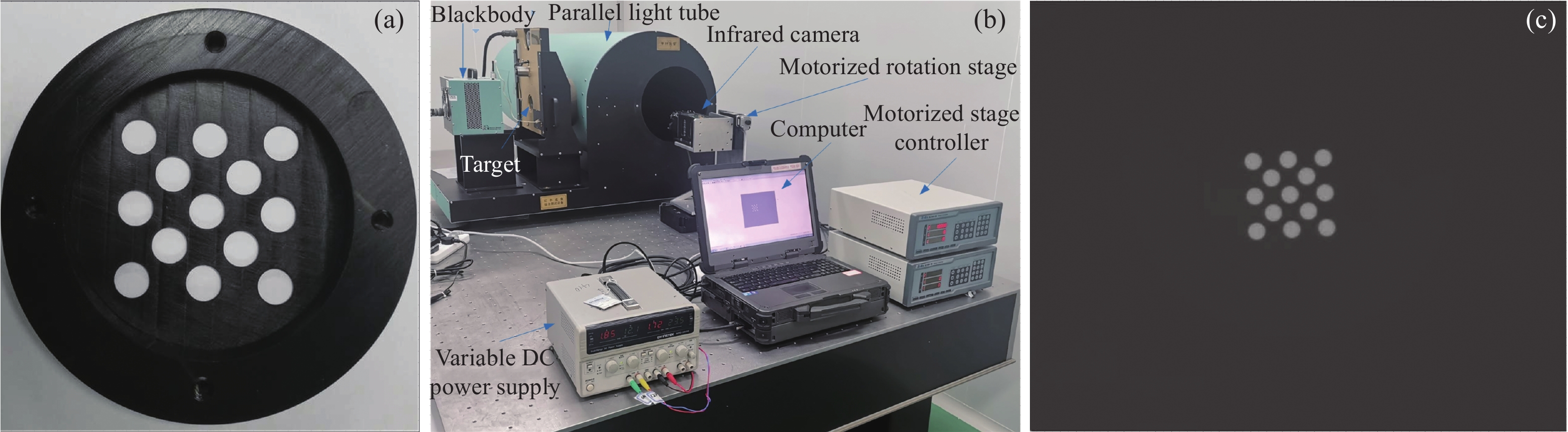
设计的靶标如图1(a)所示,由规则排列的多个圆孔组成,圆孔直径根据被测相机视场和平行光管焦距确定,使得圆孔直径在图像中为20 pixel左右。设计的靶标图案具有以下特点:圆形包含所有方向的梯度信息,可用于各向异性模糊核估计;可通过圆心检测算法精确提取圆心坐标,进而求出相机姿态,无需角点等辅助特征;根据求出的相机姿态和靶标物理尺寸,可快速生成理想高分辨率图像。
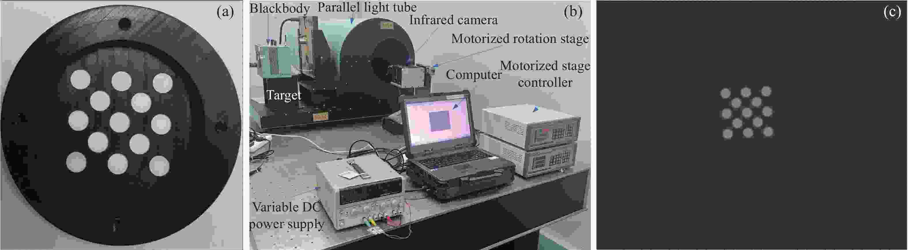
图 1 (a) 多圆孔靶标;(b) 基于平行光管的图像采集环境;(c) 实际采集的一帧靶标图像
Figure 1. (a) Multi-circle target; (b) Image acquisition environment based on parallel light tube; (c) A target image acquired by an infrared camera
靶标图像采集环境如图1(b)所示,主要由黑体、靶标、平行光管、旋转平台、被测热像仪及计算机组成。由于靶标尺寸较小,无法覆盖整个视场,因此采用旋转平台带动热像仪运动,完成扫描。实际采集的一帧靶标图像如图1(c)所示。
-
如图2所示,分别建立图像坐标系和靶标坐标系。利用OpenCV圆心检测算法计算图像中圆心$ {p}_{1} $~$ {p}_{13} $的像素坐标$ \left({u}_{1},{v}_{1}\right) $~$ \left({u}_{13},{v}_{13}\right) $;根据靶标物理尺寸,得到对应圆心${p}_{1}{'}$~${p}_{13}{'}$的物理坐标$ \left({x}_{1},{y}_{1}\right) $~$ \left({x}_{13},{y}_{13}\right) $。则图像坐标与物理坐标之间的变换矩阵H可通过公式(4)计算求得。
图 2 (a) 图像坐标系;(b) 靶标坐标系
Figure 2. (a) Image coordinate system; (b) Target coordinate system
$$ \left[\begin{array}{ccc}{u}_{1}& \dots & {u}_{13}\\ {v}_{1}& \dots & {v}_{13}\\ 1& \dots & 1\end{array}\right]=\boldsymbol{H}\left[\begin{array}{ccc}{x}_{1}& \dots & {x}_{13}\\ {y}_{1}& \dots & {y}_{13}\\ 1& \dots & 1\end{array}\right] $$ (4) 基于求出的单应矩阵H生成理想高分辨率图像的过程如下:遍历高分辨率图像中的像素坐标(uHR, vHR),计算其在低分辨率图像中的像素坐标(uLR, vLR):
$$ \left[\begin{array}{c}{u}^{\mathrm{L}\mathrm{R}}\\ {v}^{\mathrm{L}\mathrm{R}}\end{array}\right]=\left[\begin{array}{c}\dfrac{{u}^{\mathrm{H}\mathrm{R}}}{s}-\dfrac{1}{2}+\dfrac{1}{2s}\\ \dfrac{{v}^{\mathrm{H}\mathrm{R}}}{s}-\dfrac{1}{2}+\dfrac{1}{2s}\end{array}\right] $$ (5) 式中:s为超分辨倍率;${u}^{\mathrm{H}\mathrm{R}}\in [0,s\times w);{v}^{\mathrm{H}\mathrm{R}}\in [0,s\times h) $。根据单应矩阵H计算$ {(u}^{\mathrm{L}\mathrm{R}},{v}^{\mathrm{L}\mathrm{R}}) $对应的物理坐标$ (x,y) $:
$$ \left[\begin{array}{c}x\\ y\\ 1\end{array}\right]={\boldsymbol{H}}^{-1}\left[\begin{array}{c}{u}^{\mathrm{L}\mathrm{R}}\\ {v}^{\mathrm{L}\mathrm{R}}\\ 1\end{array}\right] $$ (6) 根据物理坐标$ (x,y) $判断该点位于圆内还是圆外,进行灰度赋值。
分别以圆心$ {p}_{4} $、$ {p}_{5} $、$ {p}_{9} $、$ {p}_{10} $为中心,以$ {p}_{4} $与$ {p}_{5} $间距的1.5倍为边长,截取方形图像区域,每个区域基本包含五个完整的圆形,用于求解该区域的模糊核。
-
1) 模糊核求解网络
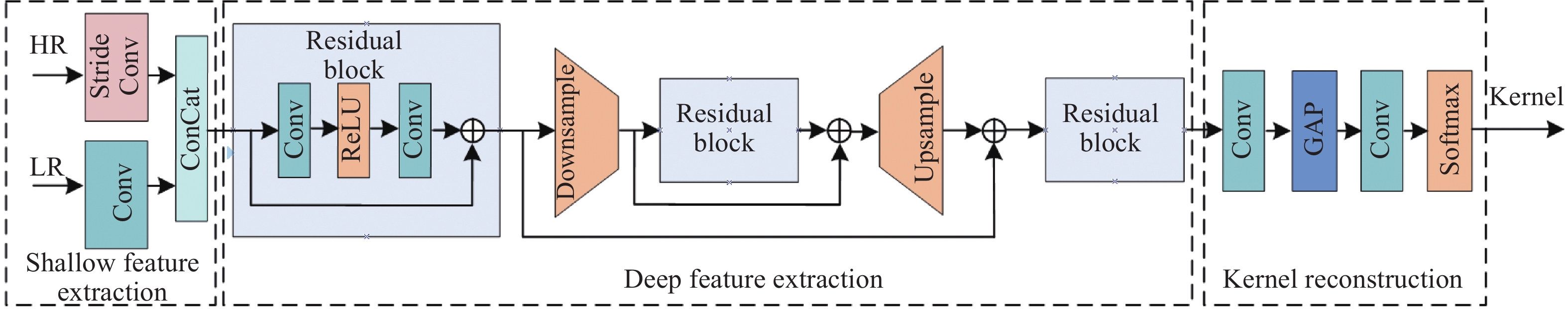
设计模糊核求解网络用于模糊核求解。网络结构如图3所示,主要由浅层特征提取模块、深层特征提取模块和模糊核估计模块三部分组成。尺寸为H×W的低分辨率图像与步长为1、大小为5×5的卷积核做卷积后,输出尺寸为32×H×W的特征;尺寸为 sH×sW的高分辨率图像与步长为s(超分辨率倍数)、大小为(4s+1)×(4s+1)的卷积核做卷积后,输出尺寸为32×H×W的特征;经过维度拼接,得到64×H×W的浅层特征表示。深层特征提取采用Unet网络结构,主要由残差模块、下采样模块和上采样模块组成。输入的浅层特征先经过残差模块处理得到尺寸为128×H×W 的特征,然后与步长为2的卷积核做卷积实现下采样,得到尺寸为$256 \times \dfrac{H}{2}\times \dfrac{W}{2}$的特征;再经过残差模块处理后,利用转置卷积模块实现上采样,得到尺寸为128× H×W的特征;最后经过残差模块处理得到尺寸为128×H×W的深层特征表示。模糊核重建模块基于深层特征重建模糊核。输入特征与3×3的卷积核做卷积后,再利用全局平局池化对特征运算结果进行融合,得到尺寸为128×1×1的融合结果;最后通过与1×1的卷积核做卷积和Softmax函数激活,输出尺寸为${ (2 r+1)}^{2} \times 1\times 1$的向量,再重排列为(2r+1)×(2r+1)(模糊核的尺寸)的张量,输出估计的模糊核。

图 3 模糊核估计网络结构
Figure 3. Overall architecture of proposed blur kernel estimation network
2) 训练数据生成
模糊核估计网络利用基于退化模型生成的高/低分辨率图像对网络进行端到端的有监督训练。与常规方法采用高分辨率图像数据集进行训练不同,文中采用仿真生成靶标类型的图像进行训练。仿真图像生成的原理与1.2.2节高分辨率图像生成原理相同,区别是单应变换矩阵依据随机生成的相机姿态角和相机焦距计算得到,计算公式如下:
$$ {{\boldsymbol{H}}}_{t}={{\boldsymbol{K}}}_{v}{{{\boldsymbol{R}}}_{rot}{\boldsymbol{R}}}_{el}{{\boldsymbol{R}}}_{az} $$ (7) 式中:${{\boldsymbol{R}}}_{az}$、${{\boldsymbol{R}}}_{el}$和${{\boldsymbol{R}}}_{rot}$分别为虚拟相机的航向、俯仰和横滚三个姿态角对应的旋转矩阵,航向角、俯仰角在(−10°, 10°)内均匀分布,横滚角在(−5°, 5°)内均匀分布;${{\boldsymbol{K}}}_{v}$为虚拟相机的内参矩阵。
$${{\boldsymbol{K}}_v} = \left[ {\begin{array}{*{20}{c}} {{f_x}}&{0}&{{W {_t}/{2}\;}}\\ {0}&{f_y}&{{H {_t}/{2}\;}}\\ {0}&{0}&{1} \end{array}} \right]$$ (8) 式中:$ {f}_{x} $、$ {f}_{y} $为焦比,通过对被测热像仪焦比增加10%的随机误差得到;${H}_{t}\times {W}_{t}$为生成图像的分辨率。
对仿真生成的高分辨率图像采用各项异性高斯模糊核进行模糊处理,并进行s倍下采样,最后加入随机噪声,得到低分辨率图像。其中噪声为加性高斯白噪声,噪声标准差在(0, 7.65)之间均匀分布。各向异性高斯模糊核的分布符合均值为0、协方差矩阵为Σ的高斯概率密度函数:
$$ k\left(i,j\right)=\frac{1}{N}\mathrm{exp}\left(-\frac{1}{2}{{\boldsymbol{C}}}^{{\rm{T}}}{{\boldsymbol{\varSigma }}}^{-1}{\boldsymbol{C}}\right),\:{\boldsymbol{C}}=\left[\begin{array}{c}i\\ j\end{array}\right] $$ (9) 式中:N为归一化参数,模糊核的尺寸为(2r+1)×(2r+1);C为空间坐标,$i,j\in [-r,r]$;Σ为协方差矩阵。
$$ {{\boldsymbol{\varSigma}} }=\left[\begin{array}{cc}{\rm{cos}}\theta & -{\rm{sin}}\theta \\ {\rm{sin}}\theta & {\rm{cos}}\theta \end{array}\right]\left[\begin{array}{cc}{\lambda }_{1}^{2}& 0\\ 0& {\lambda }_{2}^{2}\end{array}\right]\left[\begin{array}{cc}{\rm{cos}}\theta & {\rm{sin}}\theta \\ -{\rm{sin}}\theta & {\rm{cos}}\theta \end{array}\right] $$ (10) 式中:$ {\lambda }_{1} $、$ {\lambda }_{2} $为特征值,在(0.6~10)之间均匀分布;$ \theta $为旋转角度,在(0~π)之间均匀分布;$ {\downarrow }_{s} $采用双三次插值下采样。实际训练时模糊核的尺寸设为21×21。
按照上述模型生成配对的高/低分辨率图像用于训练,在4倍超分辨率时,高分辨率图像的尺寸分别为256 pixel×256 pixel,低分辨率图像的尺寸固定为64 pixel×64 pixel。通过随机旋转和翻转进行数据扩增,训练时批大小设为32。
3) 损失函数
损失函数定义为网络输出的模糊核${{\boldsymbol{k}}}_{i}$与真实模糊核${{\boldsymbol{k}}}_{{g}{t}}$之间的$ {L}_{1} $损失。
-
超分辨率重建算法原理如图4所示。依据模糊核位置,将图像分为m×n的重叠子块,每个子块大小为128 pixel×128 pixel,相邻子块之间有一定像素的重叠。将图像子块和该子块对应的模糊核及噪声标准差一起输入非盲超分辨率重建网络USRNet[15] ,得到超分辨率重建后的子块,去除边界后仅保留中心120 pixel×120 pixel的区域;对子块进行基于重叠区域欧式距离的图像融合,再通过图像合并得到最终的超分辨率图像。

图 4 超分辨率重建原理
Figure 4. Schematic diagram of super-resolution reconstruction
-
图5(a)和5(b)所示分别为两款红外热像仪采集并截取的不同位置的靶标图像及利用高分辨率图像生成算法生成的配对高分辨率图像。从图中可以看出,同一款热像仪不同区域的图像模糊特性存在一定差异;不同热像仪之间差异更加明显。
图 5 截取的长焦热像仪(a)和短焦热像仪(b)采集的靶标图像及生成的高分辨率图像
Figure 5. (a) Cropped portions of the images captured by long-focus infrared camera (a) and short-focus infrared camera (b) and synthesized high-resolution image
将高/低分辨率靶标图像输入模糊核估计网络,得到对应区域的模糊核。遍历所有图像块,得到图6(a)和6(b)所示长焦热像仪和短焦热像仪在4倍超分辨率重建时的模糊核的估计结果(为便于观测,将模糊核放大两倍显示)。
从图6中可以看出,不同镜头模糊核差异较大;靠近视场中心模糊核较小,靠近边缘模糊核较大;中心区域模糊核更加趋于各向同性,边缘区域模糊核各向异性的特征比较明显。
图 6 长焦热像仪(a)和短焦热像仪(b)模糊核估计结果
Figure 6. Estimated blur kernels of long-focus infrared camera (a) and short-focus infrared camera (b)
-
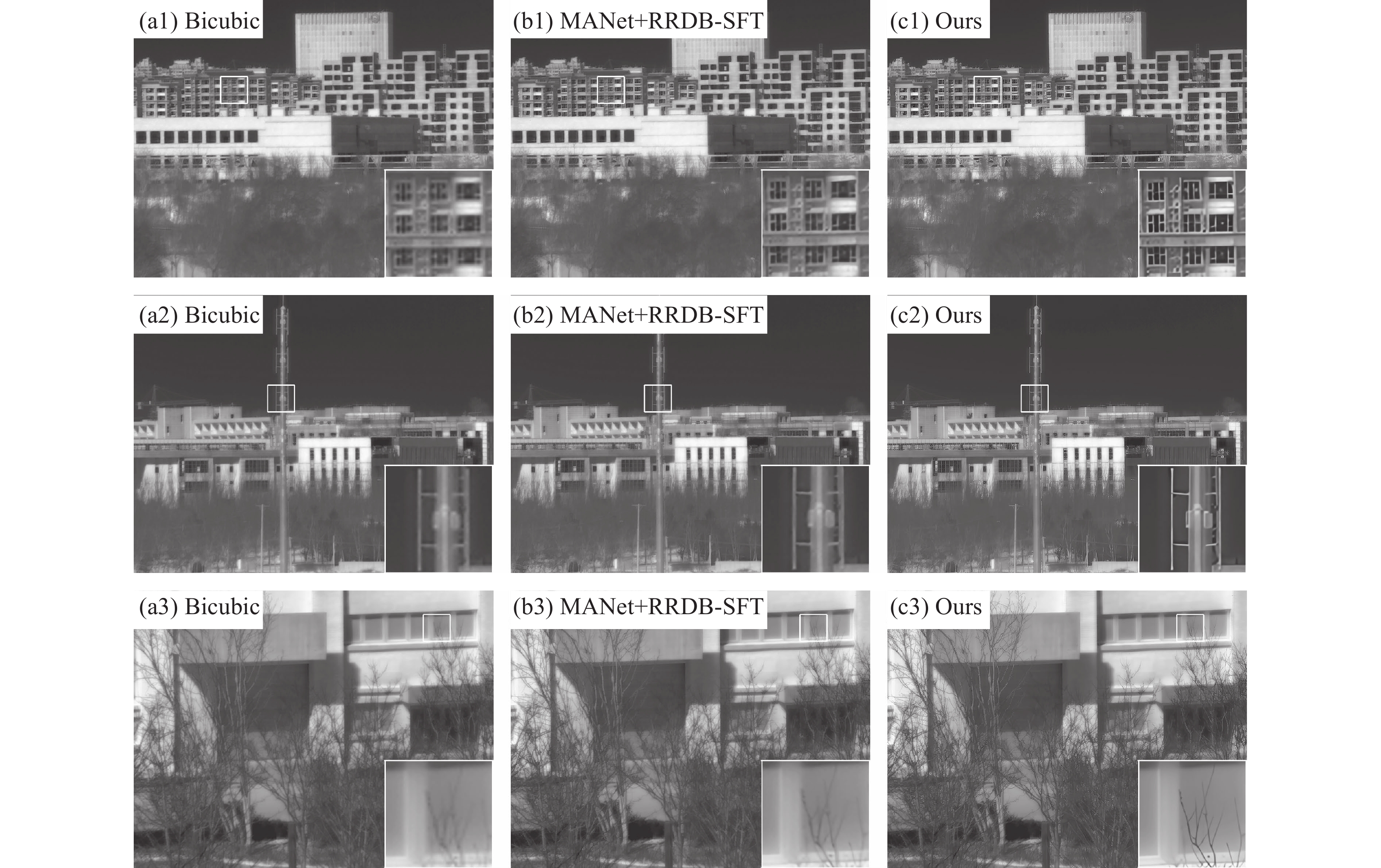
利用两款不同焦距的红外热像仪采集实际场景图像,利用标定出的模糊核和文中超分辨率重建方法进行4倍超分辨率重建,并与Bicubic上采样算法和MANet+RRDB-SFT[14] 算法进行直观对比,部分实验对比结果如图7和图8所示。
图 7 对长焦红外热像仪实际采集图像进行4倍超分辨率重建的效果对比
Figure 7. Visual results of different methods on real-world images captured by long-focus infrared camera for scale factor 4
从图7和图8中可以看出,采用Bicubic方法重建出的图像边缘比较模糊,细节难以分辨;采用MANet+RRDB-SFT方法重建的图像在强边缘处更加清晰,但弱纹理区重建效果欠佳;采用文中方法得到的重建图像边缘锐度更高,弱纹理也更清晰。

图 8 对短焦红外热像仪实际采集图像进行4倍超分辨率重建的效果对比
Figure 8. Visual results of different methods on real-world images captured by short-focus infrared camera for scale factor 4
为了更加客观地评价超分辨率重建效果,采用自然度图像质量评估模型(NIQE)、基于感知的图像质量评估模型(PIQE)和盲/无参考图像空间质量评估模型(BRISQUE)三种无参考图像质量评价方法对超分辨率重建后的图像进行客观评价,统计平均结果如表1所示。从表中可以看出,文中方法在三个客观指标上的表现都优于对比方法。
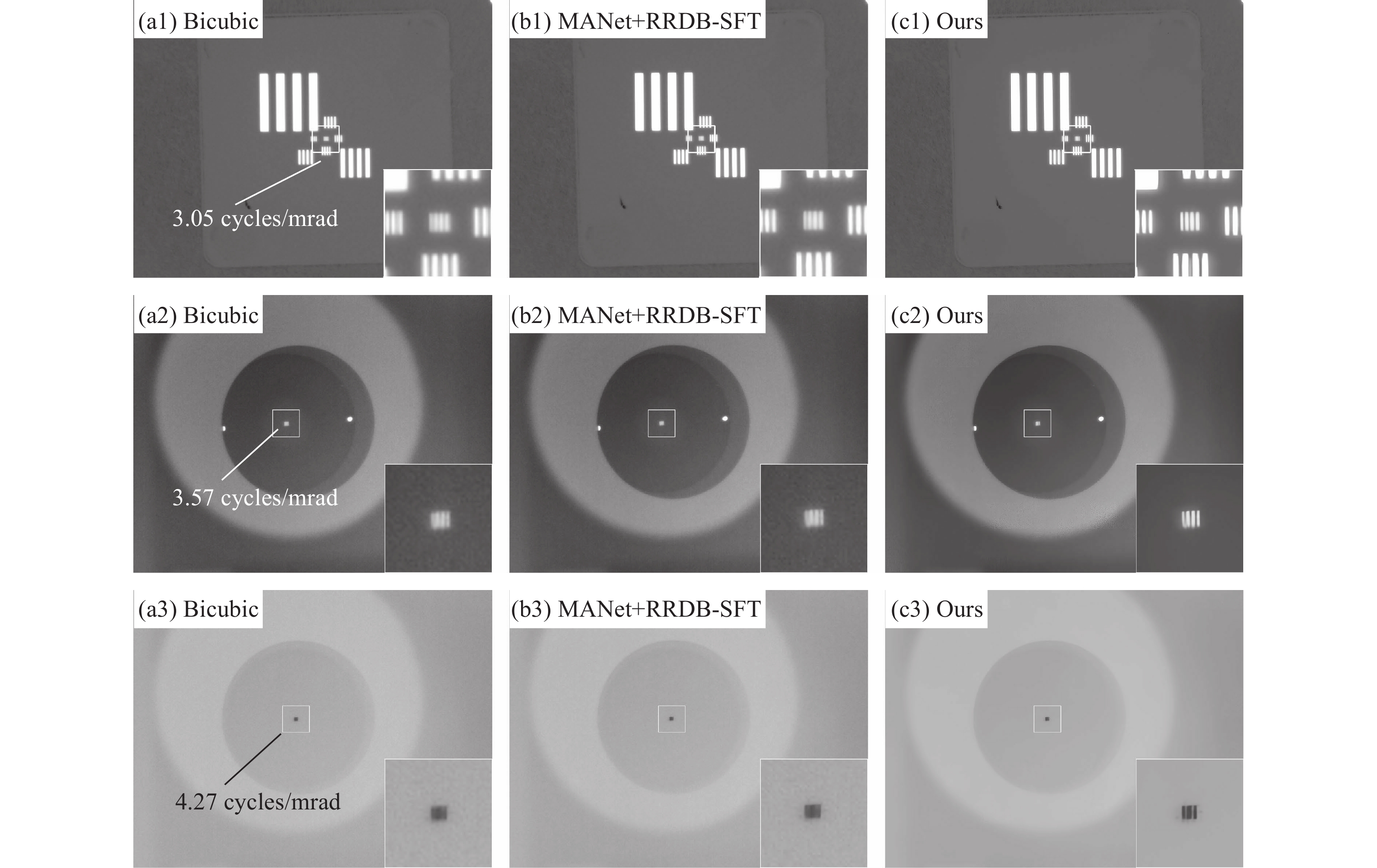
利用条带靶进一步测试文中方法对极限空间频率目标的分辨能力。利用特征频率为3.05 cycles/mrad的长焦热像仪,采集空间频率为3.05、3.57、4.27 cycles/mrad的靶标图像,并进行超分辨率重建,重建结果如图9所示。Bicubic方法和MANet+RRDB-SFT方法可基本分清3.05 cycles/mrad的靶标,而3.57 cycles/mrad的的靶标则比较模糊,难以分辨。文中方法可清晰分辨出3.57 cycles/mrad的靶标。对于4.27 cycles/mrad的靶标,由于原始图像混叠严重,Bicubic方法和MANet+RRDB-SFT方法无法重建出靶标,文中方法可重建出三条靶标。实验表明,文中方法可提高空间频率分辨能力17%以上。
表 1 不同方法4倍超分辨率重建客观评价指标对比
Table 1. Quantitative comparison with other methods with scale factor 4
Method NIQE↓ PIQE↓ BRISQUE↓ Bicubic 6.058 89.936 53.372 MANet+
RRDB-SFT4.886 83.852 52.723 Ours 4.574 82.948 49.394 
图 9 对长焦红外热像仪采集的4条靶图像进行4倍超分辨率重建效果对比
Figure 9. Visual results of different methods on 4-bar target image captured by long-focus infrared camera for scale factor 4
-
1) 复杂度评估
算法各步骤的参数量和运行时间如表2所示,测试条件为Intel Core i7-10700 CPU,Nvidia GeForce 2080Ti GPU,Ubantu20.04操作系统。高分辨率靶标图像生成算法通过Python实现,模糊核估计网络和超分辨率重建网络采用PyTorch 1.12深度学习框架。原始图像分辨率为640 pixel×512 pixel,超分辨率重建倍率为4。
表 2 算法各步骤参数量和运算时间
Table 2. Total number of parameters and runtime of each step
Step Params/M Runtime/s HR target im synthesis - 67.318 Blur kernel estimation 2.33 1.148 Super-resolution reconstruction 17.016 22.645 对于实时性要求较高的应用场景,也可单独使用文中的模糊核标定方法进行模糊核标定,然后将标定出的模糊核输入轻量级非盲超分辨率重建网络,提高实时性。
2) 局限性分析
基于标定的模糊核求解方法可获得准确的模糊核估计结果,因此重建图像的边缘锐度较高,整体更加清晰,取得了较好的视觉效果,且一定程度上提升了红外成像设备的空间频率分辨能力。但对于图像中部分对比度较低的边缘和灰度差较小的区域,存在重建后图像边缘对比度过高、灰度差被放大的现象,如何在提高图像边缘锐度的同时保持对比度基本稳定,是算法后续的改进方向。
3) 适用性分析
基于多圆孔靶的模糊核标定方法具有较高的通用性,对于任意红外成像设备,仅需采集一组覆盖图像各区域的多圆孔靶标图像即可通过文中算法完成空间非一致模糊核估计,工作量较小,工程应用中易于实现,具有较高的实际应用价值。
由于红外光学系统存在热离焦现象,环境温度变化时模糊核也会发生改变。通过光学系统无热化设计可有效降低环境温度的影响,但并不能完全消除。可利用模糊核与环境温度之间关系相对固定这一特点,标定出不同环境温度下的模糊核,并存储在成像系统中。使用时,依据环境温度选择合适的模糊核进行超分辨率重建。如何建立模糊核随环境温度变化模型,或设计寻优算法,基于少量标定数据实时估计模糊核,从而进一步降低标定工作量,是文中后续研究的主要内容。
-
文中提出了一种基于标定的非盲模糊核估计方法,通过采集特定靶标图像并设计模糊核估计网络,标定出空间非一致模糊核,并设计基于图像分块的超分辨率重建方法,实现空间非一致模糊图像重建。实验结果表明,光学系统自身引起的模糊随空间位置变化相对缓慢,因此可对一定图像区域估计一个模糊核,无需稠密估计,从而降低了标定复杂度和超分辨率重建时的数据量。基于标定出的模糊核和图像分块的超分辨率重建方法可显著提高超分辨率重建效果。此外,所提出的方法工作量较小,具有较高的工程应用价值。后续将针对算法存在的部分弱边缘重建后对比度变化较大的问题进行算法改进;针对热离焦导致的模糊核变化问题进行深入研究,扩展方法的适用范围。
Infrared image super-resolution based on spatially variant blur kernel calibration
-
摘要: 近年来,红外成像系统在工业、安防、遥感等领域获得了广泛的应用,但由于制造工艺及成本制约,红外系统的分辨率仍然较低。基于深度神经网络的单帧图像超分辨率重建技术是提高红外图像分辨率的有效方法,获得了广泛研究,并在仿真图像上取得了显著进展,但应用于实际场景图像时容易出现伪影或图像模糊等现象。造成这种性能差异的主要原因是目前方法大多假定造成图像退化的模糊核是空间一致的,然而实际红外光学系统不可避免地存在像差、热离焦等,由此造成的图像模糊的模糊核并非空间一致的。针对这一问题,提出了一种非盲模糊核估计方法,通过采集特定的靶标图像,并设计模糊核估计网络,求解空间非一致模糊核;设计基于图像分块的超分辨率重建方法,将图像块和对应区域的模糊核一起输入非盲超分辨率重建网络进行子块图像重建,再通过子块合并和重叠区域图像融合,得到最终的高分辨率图像。实验结果表明,光学系统自身引起了模糊核随空间位置缓慢变化,在实验室条件下标定模糊核并基于图像分块进行超分辨率重建的方法可显著提高红外图像超分辨率重建的效果。Abstract:
Objective In recent years, infrared imaging systems have been increasingly used in industry, security, and remote sensing. However, the resolution of infrared devices is still quite limited due to its cost and manufacturing technology restrictions. To increase image resolution, deep learning-based single image super-resolution (SISR) has gained much interest and made significant progress in simulated images. However, when applied to real-world images, most approaches suffer a performance drop, such as over-sharpening or over-smoothing. The main reason is that these methods assume that blur kernels are spatially invariant across the whole image. But such an assumption is rarely applicable for infrared images, whose blur kernels are usually spatially variant due to factors such as lens aberrations and thermal defocus. To address this issue, a blur kernel calibration method is proposed to estimate spatially-variant blur kernels, and a patch-based super-resolution (SR) algorithm is designed to reconstruct super-resolution images. Methods Parallel light tube and motorized rotating platform are used to establish target image acquisition environment, and then images of multi-circle target at different positions are gathered (Fig.1). Based on sub-pixel accurate circle center detection, the camera pose parameters are solved, and high-resolution target images are synthesized according to the parameters. High-resolution and low-resolution target image pairs are fed into the blur kernel estimation network to obtain accurate blur kernels (Fig.3). In addition, a patch-based super-resolution algorithm is designed, which decomposes the test image into overlapping patches, reconstructs each of them separately using estimated kernels, and finally merges them according to Euclidean distances (Fig.4). Results and Discussions The experimental results show that the blur caused by the optical system is not negligible and varies slowly with spatial position (Fig.6). The proposed method, which calibrates blur kernels in a laboratory setting, can obtain a more accurate blur kernel estimation result. As a consequence, the proposed patch-based super-resolution algorithm can produce more visually pleasant results with more reliable details (Fig.7-8), and can also boost objective quality evaluation indicators such as natural image quality evaluator (NIQE), perception based image quality evaluator (PIQE), and blind/referenceless image spatial quality evaluator (BRISQUE) (Tab.1). SR experiments on 4-bar targets with different spatial frequencies show that the proposed method can distinguish the target with spatial frequency of 3.57 cycles/mrad, while comparison methods can just distinguish that of 3.05 cycles/mrad under the same conditions (Fig.9). Conclusions A blur kernel calibration method is proposed to estimate spatially-variant blur kernels, and a patch-based super-resolution algorithm is designed to implement super-resolution reconstruction. The experimental results show that image blur caused by the optical system changes slowly with the spatial position. As a result, one blur kernel can be estimated for each image patch, instead of densely estimated for each pixel, thereby reducing the complexity of calibration and memory consumption during reconstruction. Thanks to the accurate blur kernel estimation, the proposed super-resolution algorithm outperforms the comparison methods in both qualitative and quantitative results. Furthermore, the blur kernel calibration method is easy to implement in engineering applications. For any infrared camera, only dozens of multi-circle target images covering all areas of the focal plane are needed to complete the calibration process. When real-time performance is required, the proposed blur kernel calibration method can also be combined with other lightweight non-blind super-resolution methods to achieve a real-time performance. In the future, the problem of image blur caused by thermal defocusing will be studied to expand the scope of the method. -
图 1 (a) 多圆孔靶标;(b) 基于平行光管的图像采集环境;(c) 实际采集的一帧靶标图像
Figure 1. (a) Multi-circle target; (b) Image acquisition environment based on parallel light tube; (c) A target image acquired by an infrared camera
图 2 (a) 图像坐标系;(b) 靶标坐标系
Figure 2. (a) Image coordinate system; (b) Target coordinate system
图 3 模糊核估计网络结构
Figure 3. Overall architecture of proposed blur kernel estimation network
图 5 截取的长焦热像仪(a)和短焦热像仪(b)采集的靶标图像及生成的高分辨率图像
Figure 5. (a) Cropped portions of the images captured by long-focus infrared camera (a) and short-focus infrared camera (b) and synthesized high-resolution image
图 6 长焦热像仪(a)和短焦热像仪(b)模糊核估计结果
Figure 6. Estimated blur kernels of long-focus infrared camera (a) and short-focus infrared camera (b)
图 7 对长焦红外热像仪实际采集图像进行4倍超分辨率重建的效果对比
Figure 7. Visual results of different methods on real-world images captured by long-focus infrared camera for scale factor 4
图 8 对短焦红外热像仪实际采集图像进行4倍超分辨率重建的效果对比
Figure 8. Visual results of different methods on real-world images captured by short-focus infrared camera for scale factor 4
图 9 对长焦红外热像仪采集的4条靶图像进行4倍超分辨率重建效果对比
Figure 9. Visual results of different methods on 4-bar target image captured by long-focus infrared camera for scale factor 4
表 1 不同方法4倍超分辨率重建客观评价指标对比
Table 1. Quantitative comparison with other methods with scale factor 4
Method NIQE↓ PIQE↓ BRISQUE↓ Bicubic 6.058 89.936 53.372 MANet+
RRDB-SFT4.886 83.852 52.723 Ours 4.574 82.948 49.394  下载: 导出CSV
表 2 算法各步骤参数量和运算时间
Table 2. Total number of parameters and runtime of each step
Step Params/M Runtime/s HR target im synthesis - 67.318 Blur kernel estimation 2.33 1.148 Super-resolution reconstruction 17.016 22.645
下载: 导出CSV
-
[1] Dong C, Loy C C, He K, et al. Learning a deep convolutional network for image super-resolution [C]//European Conference on Computer Vision. Cham: Springer, 2014: 184-199. [2] Kim J, Lee J K, Lee K M. Deeply-recursive convolutional network for image super-resolution [C]//Proceedings of the IEEE Conference on Computer Vision and Pattern Recognition, 2016: 1637-1645. [3] Lim B, Son S, Kim H, et al. Enhanced deep residual networks for single image super-resolution [C]//Proceedings of the IEEE Conference on Computer Vision and Pattern Recognition Workshops, 2017: 136-144. [4] Zhang Y, Li K, Li K, et al. Image super-resolution using very deep residual channel attention networks [C]//Proceedings of the European Conference on Computer Vision (ECCV), 2018: 286-301. [5] 张秀, 周巍, 段哲民, 魏恒璐. 基于卷积稀疏自编码的图像超分辨率重建[J]. 红外与激光工程, 2019, 48(1): 126005-0126005(7). doi: 10.3788/IRLA201948.0126005 Zhang Xiu, Zhou Wei, Duan Zhemin, et al. Convolutional sparse auto-encoder for image super-resolution reconstruction [J]. Infrared and Laser Engineering, 2019, 48(1): 0126005. (in Chinese) doi: 10.3788/IRLA201948.0126005 [6] 魏子康, 刘云清. 改进的RDN灰度图像超分辨率重建方法[J]. 红外与激光工程, 2020, 49(S1): 20200173-020200173(8). doi: 10.3788/IRLA20200173 Wei Zikang, Liu Yunqing. Gray image super-resolution reconstruction based on improved RDN method [J]. Infrared and Laser Engineering, 2020, 49(S1): 20200173. (in Chinese) doi: 10.3788/IRLA20200173 [7] Liu A, Liu Y, Gu J, et al. Blind image super-resolution: A survey and beyond [J]. IEEE Transactions on Pattern Analysis and Machine Intelligence, 2023, 45(5): 5461-5480. doi: 10.1109/TPAMI.2022.3203009 [8] Gu J, Lu H, Zuo W, et al. Blind super-resolution with iterative kernel correction [C]//Proceedings of the IEEE/CVF Conference on Computer Vision and Pattern Recognition, 2019: 1604-1613. [9] Bell-Kligler S, Shocher A, Irani M. Blind super-resolution kernel estimation using an internal-gan [C]//Advances in Neural Information Processing Systems, 2019: 284-293. [10] Liang J, Zhang K, Gu S, et al. Flow-based kernel prior with application to blind super-resolution [C]//Proceedings of the IEEE/CVF Conference on Computer Vision and Pattern Recognition, 2021: 10601-10610. [11] Joshi N, Szeliski R, Kriegman D J. PSF estimation using sharp edge prediction [C]//2008 IEEE Conference on Computer Vision and Pattern Recognition. IEEE, 2008: 1-8. [12] Kee E, Paris S, Chen S, et al. Modeling and removing spatially-varying optical blur [C]//2011 IEEE International Conference on Computational Photography (ICCP). IEEE, 2011: 1-8. [13] Cai J, Zeng H, Yong H, et al. Toward real-world single image super-resolution: A new benchmark and a new model [C]//Proceedings of the IEEE/CVF International Conference on Computer Vision, 2019: 3086-3095. [14] Liang J, Sun G, Zhang K, et al. Mutual affine network for spatially variant kernel estimation in blind image super-resolution [C]//Proceedings of the IEEE/CVF International Conference on Computer Vision, 2021: 4096-4105. [15] Zhang K, Gool L V, Timofte R. Deep unfolding network for image super-resolution [C]//Proceedings of the IEEE/CVF Conference on Computer Vision and Pattern Recognition, 2020: 3217-3226. -

 点击查看大图
计量
- 文章访问数: 158
- HTML全文浏览量: 24
- PDF下载量: 43
- 被引次数: 0

