


 下载:
下载:

-
自由曲面是一种不具有旋转对称或平移对称的光学曲面,其灵活的面型结构为设计者提供了极高的设计自由度。相较于传统的球面和非球面,自由曲面可以实现更为复杂的光束调控功能,并且得到更为紧凑的光学系统[1],被广泛应用于车灯照明[2-3]、显微照明[4-5]、内窥照明[6]、激光光束整形[7-9]、近眼显示AR等[10-11]领域。
自由曲面光束调控通常包括对出射光强的调控以及对出射光强和波前形状的同时调控,文中主要研究对出射光强和波前的同时调控。对光束强度和波前的同时调控通常表示为经自由曲面透镜后的出射光束具有预定的波面形状,如平面波、球面波等,同时能够在目标面上形成特定的强度或者照度分布。2013年,Feng等人[12]采用光线映射(Ray-mapping)方法设计了同时调控输出光束的辐射照度分布和波前分布的双平面-自由曲面透镜,该方法可以将一束准直的高斯光束在垂轴目标面上整形成景深长、发散角小的均匀矩形光束,同时整形后的波前为平面波。该方法只考虑一个点的斜率来计算第一个自由曲面上的下一个点,会产生一定的表面构造误差。同年,Feng等人[13]开发了一种改进方法来构造两个误差较小的自由曲面,得到目标面上规定的辐照度分布RMS误差比之前减小了25.7%,但其采用的映射方法只有在近轴近似下才能满足可积性条件。2014年,Zhang等人[14]基于Monge-Ampère (MA)方程法构建了适用于将准直入射光调控为准直出射光且有预定照度分布的模型,实现了将具有高斯分布的入射光调均匀分布或具有图案分布的准直出射光。2019年,Wei等人[15]提出了一种不受平面或球面入射波限制的双光滑自由曲面设计方法,来控制光束的辐照度和相位,与传统的光线映射方法相比,该方法将光线映射的计算和自由曲面的构造相结合,有效解决了光束整形的光线映射可积性问题。2020年,Mingazov等人[16]针对入射和出射光束是平面波的情况,提出一种基于SQM的准直光束整形方法,并且将准直的入射光束整形为准直的出射光束,出射光束为均匀的方形光斑分布或者非均照度的环形光斑。2020年,Yang等人[6]采用MA方法实现了在对光束波前和强度的同时调控,实现了在垂轴目标面上的均匀的方形分布,并且出射波前为球面波。2021年,Bykov[17]等人采用SQM方法实现了将平面波入射光调控为同时具有目标照度分布的非平面波出射光,实现了将均匀平面入射光束在目标面上形成在方框区域具有均匀辐照度分布和复杂的eikonal函数形式波前分布的光束。
上述自由曲面光束强度与波前调控方法依赖于垂轴光路布局,即要求观测目标平面与光轴垂直,这无疑制约了自由曲面光束强度与波前调控的广泛应用,例如在激光整形、AR近眼显示等领域,离轴的光路布局将得到更紧凑的光学系统。为了获得灵活的光路布局,文中在垂轴光束强度与波前调控的基础上,通过将观测平面的空间位姿纳入光束调控,打破了垂轴光路布局制约,在非垂轴的观测平面上实现了对理想点光源出射光束的波前和强度的灵活调控。
-
在前期研究中,笔者课题组已建立了垂轴光路布局下的自由曲面光束强与波前调控方法[6],在该工作的基础上,文中将采用自由曲面在非垂轴观测平面上实现光束强度与波前的同时调控。光束强度与波前的同时调控至少需要两个自由曲面,即透镜的入射面和出射面均为自由曲面,且其关键点在于如何将光强与波前同时约束,并且将观测平面的空间位姿纳入到自由曲面设计。文中首先结合斯涅尔定律、能量守恒定律以及光程约束条件构建了对波前和光强进行同时调控的光束调控模型。之后针对目标平面的非垂轴布局,通过引入垂轴虚拟平面,结合预定的波前形状以及能量守恒定律建立了离轴目标面与垂轴虚拟面上的能量分布的映射关系。最后,根据该映射关系,通过求解光束调控模型便可得到非垂轴观测平面上光束强度与波前调控问题的数值解。
-
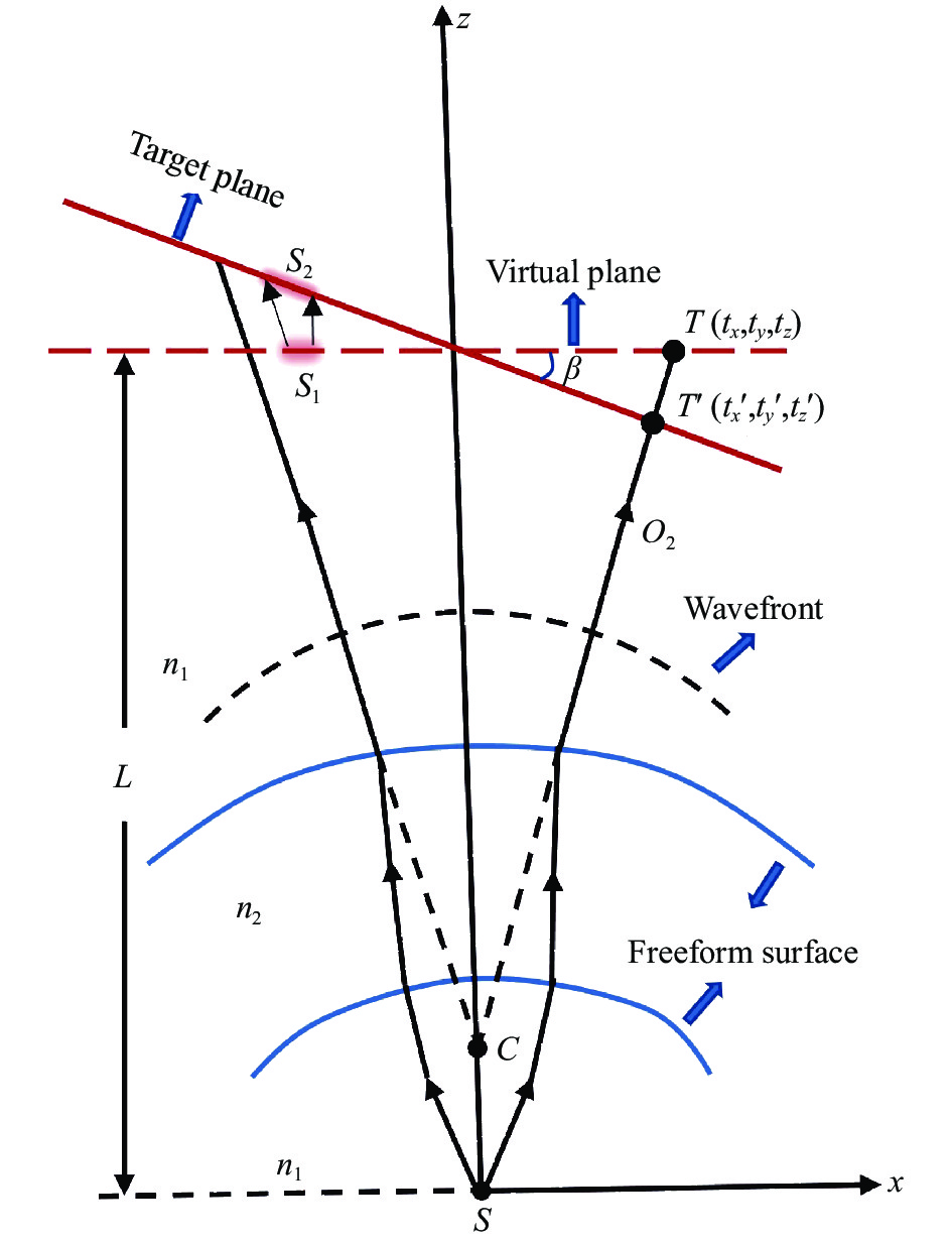
图1给出了非垂轴观测平面上自由曲面光束强度与波前调控示意图。一个可视为点光源的小尺寸光源位于xyz坐标系原点,从光源S出射任意一条光线至第一个自由曲面上一点P,经折射后到达第二个自由曲面上一点Q,再经折射后到达目标面上一点T。出射光束需在预定的倾斜平面上产生预定的辐射照度分布,同时还应具有发散的球面波,球面波中心位于光轴上一点C。需要说明的是,对于出射光束为汇聚球面波或者平面波,文中方法同样适用。ρ是P点和S点之间的距离,是一个关于方位角θ和极角φ的函数,即ρ=ρ(θ, φ)。P点的位置矢量可以表示为P=ρ∙I,其中I为入射光线的单位方向向量。根据微分几何知识,可以得到入射面上点P处的沿着θ和φ的切向量为:

图 1 基于离轴目标面的自由曲面光束强度及波前调控模型
Figure 1. Model of beam intensity and wavefront control based on an off-axis target plane using freeform surfaces
$$ \left\{ \begin{gathered} {{\boldsymbol{P}}_\theta } = {\rho _\theta } \cdot {\boldsymbol{I}} + \rho \cdot {{\boldsymbol{I}}_\theta } \\ {{\boldsymbol{P}}_\varphi } = {\rho _\varphi } \cdot {\boldsymbol{I}} + \rho \cdot {{\boldsymbol{I}}_\varphi } \\ \end{gathered} \right. $$ (1) 式中:ρθ和ρφ分别为ρ关于θ和φ的一阶偏导数;Iθ和Iφ分别为I在方向θ和φ的一阶偏导数。进一步可得,入射面在点P处的单位法向量为:
$$ {\boldsymbol{N}} = \frac{{{{\boldsymbol{P}}_\theta } \times {{\boldsymbol{P}}_\varphi }}}{{\left| {{{\boldsymbol{P}}_\theta } \times {{\boldsymbol{P}}_\varphi }} \right|}} $$ (2) 已知曲面上点P处的入射光单位方向向量和单位法向量,根据斯涅尔定律可得到点P处的出射光线的单位方向向量O1为:
$$ {n_2}{{\boldsymbol{O}}_1} = {n_1}{\boldsymbol{I}} + P \cdot {\boldsymbol{N}} $$ (3) 式中:n2为自由曲面透镜材料的折射率;n1为所处环境的折射率,一般为空气,取n1=1;$P = \sqrt {n_2^2 - n_1^2 + ({\boldsymbol{I}} \cdot {\boldsymbol{N}})} - {\boldsymbol{I}} \cdot {\boldsymbol{N}}$。进一步可将经点Q的位置矢量表示为:
$$ {\boldsymbol{Q}} = {\boldsymbol{P}} + \left| {{\boldsymbol{PQ}}} \right| \cdot {{\boldsymbol{O}}_1} $$ (4) 式中:|PQ|为矢量PQ的模,代表了点P到点Q的距离。由于从光源S发出的光束经自由曲面透镜调控后仍然是一个发散的球面波,其球心位于点C,因此,经过S点和C点的所有光线具有相同的光程,可表示为:
$$ OPL = {n_1} \cdot \left| {{\boldsymbol{SP}}} \right| + {n_2} \cdot \left| {{\boldsymbol{PQ}}} \right| - {n_1} \cdot \left| {{\boldsymbol{QC}}} \right| $$ (5) 式中:|SP|=ρ;|QC|为矢量QC的模,代表点Q到点C的距离。将公式(5)代入公式(4)可得到|PQ|的表达式,显然,|PQ|是关于ρ, θ, φ, ρθ, ρφ的函数。由此可知,在求得|PQ|后,根据公式(4)便可求得矢量Q,即出射面的坐标。利用目标面上点T、点Q、点C三者之间的几何关系可以进一步求得点T的x和y坐标,即:
$$ {t_x} = {Q_x}\frac{{{C_z} - {t_z}}}{{{C_z} - {Q_z}}} \;\;\;\;\;\;\;\;\;\;\;\;\;\;\;{t_y} = {Q_y}\frac{{{C_z} - {t_z}}}{{{C_z} - {Q_z}}} $$ (6) 式中:Qx、Qy、Qz为点Q的直角坐标分量;Cz为点C的z坐标,点C位于z轴上;tx、ty、tz为点T的直角坐标分量,若目标面为垂轴平面,此处tz便是一个常数,这将极大简化后续的推导和求解过程,而当目标面为倾斜平面时,tz则不再是一个常量,对倾斜平面的处理将在下一小节进行讨论。
由于矢量Q是关于ρ,θ, φ, ρθ, ρφ的函数,因此tx和ty也是关于ρ, θ, φ, ρθ, ρφ的函数,即:
$$ \left\{ \begin{gathered} {t_x} = {t_x}(\rho ,\;\theta ,\;\varphi ,\;{\rho _\theta },{\rho _\varphi }) \\ {t_y} = {t_y}(\rho ,\;\theta ,\;\varphi ,\;{\rho _\theta },{\rho _\varphi }) \\ \end{gathered} \right. $$ (7) 进一步假定光束在传输过程中无能量损耗,由局部能量守恒定律可得:
$$ E({t_x},{t_y})\left| {J({\boldsymbol{T}})} \right| - I(\theta ,\varphi )\sin \varphi = 0 $$ (8) 式中:E(tx, ty)为细光束在点T处产生的辐射照度;I(θ, φ)为入射细光束在θ和φ方向的光强;|J(T)|为位置矢量T的雅各比矩阵的行列式,表示为:
$$ \left| {J({\boldsymbol{T}})} \right| = \frac{{\partial {t_x}}}{{\partial \varphi }} \times \frac{{\partial {t_y}}}{{\partial \theta }} - \frac{{\partial {t_x}}}{{\partial \theta }} \times \frac{{\partial {t_y}}}{{\partial \varphi }} $$ (9) 将公式(9)代入公式(8),经过推导和化简可以得到一个椭圆型的MA方程为:
$$ A_1({\rho _{\theta \theta }}{\rho _{\varphi \varphi }} - \rho _{\theta \varphi }^2) + A_2{\rho _{\varphi \varphi }} + A_3{\rho _{\theta \theta }} + A_4{\rho _{\theta \varphi }} + A_5 = 0 $$ (10) 式中:Ai(i=1,···,5)为关于ρ, θ, φ, ρθ, ρφ的函数。公式(8)表示了入射光束的内部光线满足的能量守恒及分配约束。对于边界光线,笔者仍需要定义边界条件来保证边界光线经自由曲面偏折后到达目标光斑的边界,即边界光线需满足以下条件:
$$ \left\{ \begin{gathered} {g_x} = {g_x}(\rho ,\theta ,\varphi ,{\rho _\theta },{\rho _\varphi }) \\ {g_y} = {g_y}(\rho ,\theta ,\varphi ,{\rho _\theta },{\rho _\varphi }) \\ \end{gathered} \right., \partial {\varOmega _1} \to \partial {\varOmega _2} $$ (11) 式中:Ω1为入射光束的分布区域;Ω2为出射光束在观测平面上的分布区域;∂Ω1为Ω1的边界;∂Ω2为Ω2的边界。公式(10)和公式(11)共同构成了自由曲面光束强度与波前调控模型,这是一个带有非线性边界条件的MA方程,是一个高度的非线性方程,无法得到其解析解,只能通过离散的方式得到其数值解,此处采用有限差分法来求解该光束调控模型的数值解。
-
文中旨在解决非垂轴观测平面上自由曲面光束强度与波前调控问题,然而由于观测平面不垂直于光轴,这使得构建非垂轴观测平面上光束强度与波前调控模型变得极为困难。为了解决该光束调控问题,引入了垂轴虚拟面,并将离轴目标面上的特定照度分布映射为垂轴虚拟面上的相应照度分布,如图2所示。光束强度与波前同时调控意味着出射光束的传播方向和在目标面上的照度分布是已知的参数,此处以出射光束为发散的球面波为例, 并假定目标倾斜面为垂轴虚拟面沿y轴旋转β角度。光线在目标倾斜平面上的落点为T ′ (tx′, ty′, tz′),出射发散球面波的球心为C (Cx, Cy, Cz),则可计算得出射光线O2的xyz分量为:

图 2 离轴目标面到垂轴虚拟面的映射模型
Figure 2. Mapping model from off-axis target plane to vertical virtual plane
$$ {{\boldsymbol{O}}_{2{{x}}}} = \frac{{{t_x}' - {C_x}}}{{|{{TC}}|}},\;{{\boldsymbol{O}}_{2y}} = \frac{{{t_y}' - {C_y}}}{{|{{TC}}|}},\;{{\boldsymbol{O}}_{2z}} = \frac{{{t_z}' - {C_z}}}{{|{{TC}}|}} $$ (12) 假设垂轴目标面可表示为tz=L, 则出射光线O2与垂轴平面的交点T (tx, ty, tz)满足方程:
$$ \frac{{{t_x} - {C_x}}}{{{{\boldsymbol{O}}_{2x}}}} = \frac{{{t_y} - {C_y}}}{{{{\boldsymbol{O}}_{2y}}}} = \frac{{{t_z} - {C_z}}}{{{{\boldsymbol{O}}_{2z}}}} $$ (13) 由于Tz已知,则可根据公式(13)来求得离轴目标面上的点T ′ (tx′, ty′, tz′)映射到垂轴虚拟面上对应的坐标点T (tx, ty, tz)。
之后结合映射关系、非垂轴平面上的预定照度分布以及能量守恒定律便可计算出垂轴虚拟面上T点处的相应照度值E(tx, ty)=S2E′ (tx′, ty′)/S1,其中S1和S2分别为细光束穿过垂轴虚拟面和离轴目标面上对应小区域的面积,E(tx, ty)和E′(tx′, ty′)分别为该小区域处的照度值。
-
在该实例中,笔者的设计目标是将一个朗伯体点光源的出射光束整形为具有发散球面波前的光束,并在非垂轴目标面上形成均匀的方形照明光斑,如图3(a)所示。光源S到光轴与目标面交点W的距离SW=300 mm,自由曲面透镜的光束收集角$ \varphi $max=30°, β=30°,目标光斑的尺寸为240 mm×240 mm,目标出射光波前为发散的球面波,波前曲率中心C与光源S重合。首先采用上一节中所述的映射关系将目标倾斜平面上的照度分布映射为虚拟垂轴平面上对应的照度分布。图3(b)和图3(c)分别为映射前后的辐射照度分布图,从该图可知,这一映射关系使得光斑在形状和能量分布方面都进行了重新排列。从图3(c)中可以看出:经过映射后的光斑形状变为梯形,具有梯度变化的能量分布,并且光斑中心与光轴方向发生偏离。显然,完成这样复杂的光束能量调控,并且同时要兼顾波前形状是一个具有挑战性的问题。文中使用上述MA方程法设计自由曲面透镜,利用MA方程法可以自动满足表面连续性可积条件的优势,求解得到表面连续光滑易于加工的自由曲面面型。自由曲面的入射面和出射面的面型分布分别如图3(d)和3(e)所示,从面型图中可知计算得到的自由曲面表面形状复杂但仍然光滑连续,图3(f)所示为自由曲面透镜模型。
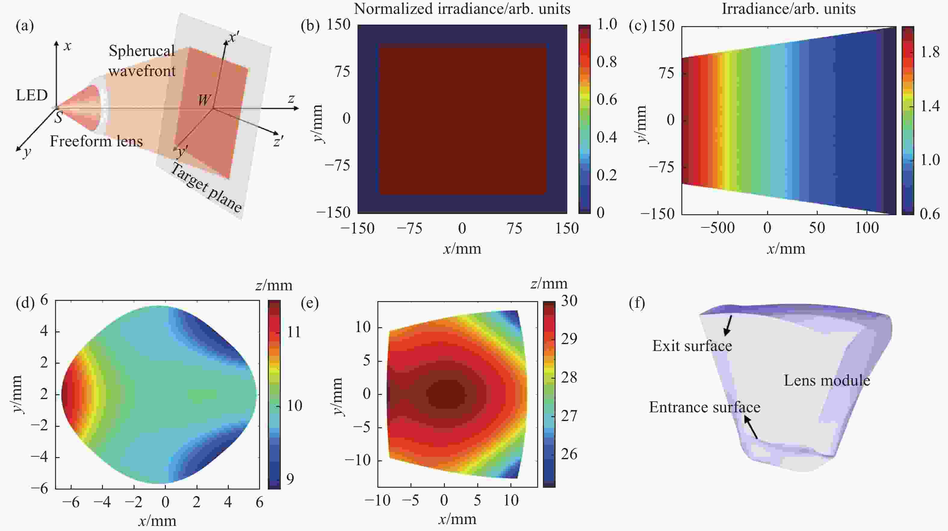
图 3 离轴面上光强和波前同时调控的设计实例。(a) 光束调控模型;(b)离轴目面上的目标照明分布;(c)映射为垂轴虚拟面上相应的照明分布;(d)入射面面型;(e)出射面面型;(f)自由曲面透镜模型
Figure 3. A design example of simultaneous control of light intensity and wavefront on off-axis plane. (a) Optical control model; (b) Target irradiance distribution of the off-axis target plane; (c) Mapping of the irradiance distribution on the vertical virtual plane; (d) Entrance surface; (e) Exit surface, and (f) the lens model
为了评价该透镜的光束调控结果,笔者追迹了1 000万条光线,仿真得到目标面上的照度分布,如图4(a)所示,其归一化照度曲线如图4(b)所示。采用公式(14)所定义的RMS[6]来表征系统的照度偏差为:
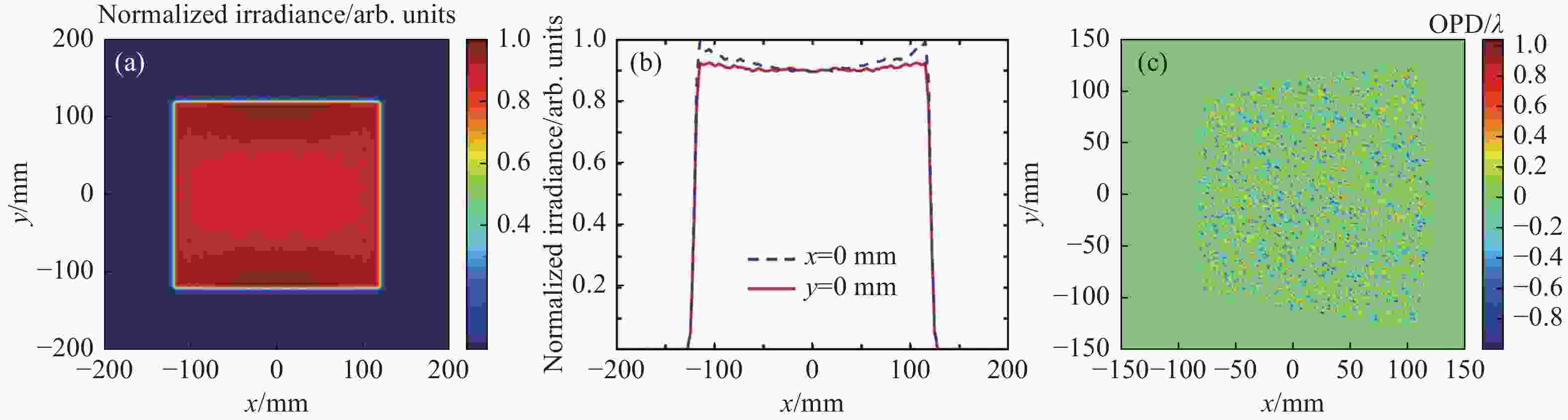
图 4 离轴目标面上照明效果的仿真验证。(a) |SW|=300 mm时倾斜目标面上的归一化照明分布;(b) |SW|=300 mm时沿着x=0 mm和y=0 mm的归一化照度曲线;(c)光程差分布
Figure 4. Simulation verification of lighting effects on the tilted target plane. (a) Normalized irradiance distribution on the tilted target plane of |SW|= 300 mm; (b) Normalized irradiance curves along the lines x=0 mm and y=0 mm; (c) Optical path difference distributions
$$ {\rm{RMS}} = \sqrt {\frac{1}{{num}}{{\sum\limits_{i = 1}^{num} {\left( {\frac{{{E_i} - {E_a}}}{{{E_a}}}} \right)} }^2}} $$ (14) 式中:Ei为目标面上照明光斑的第i个采样点处的照度值;Ea为照明光斑的平均照度值。显然,RMS值越小,则意味着实际辐射照度与目标分布偏差越小。由图4(a)可知:RMS=0.0117,表明实际辐射照度分布与目标照度分布吻合较好。由于出射光束为发散的球面波,为检测透镜对波前的调控效果,将一个球形接收面放置于W点处来计算出射光束的波前差,该球形接收面的曲率中心与目标出射球面波的球心C点重合,仿真得到实际波前分布与理想球面分布之间的光程差分布图如图4(c)所示。将图中所有的波前差分布取绝对值,再求平均值计算得到的平均波前差为0.4419λ,其中λ=541.6 nm。从仿真照度分布以及对波前误差的分析结果可知,经自由曲面透镜的调控后,入射光束的强度与波前分布均得到了很好的调控。
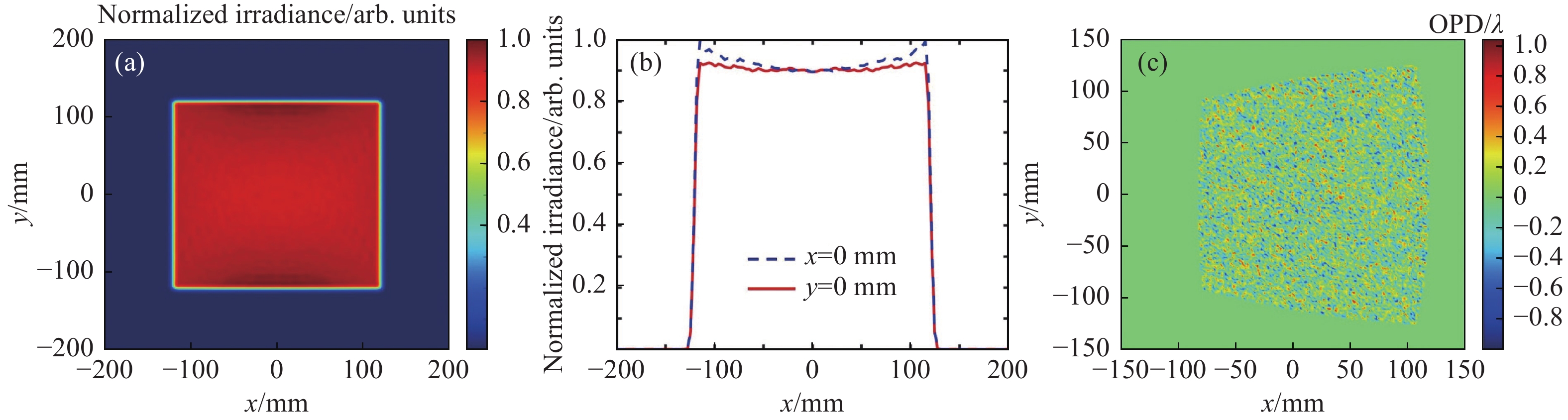
此外,在多个不同照明距离处放置接收屏来进行光线追迹,由于目标出射波前为发散的球面波,因此理论上在不同照明距离处得到的光斑形状仍然为方形,照度分布仍然为均匀分布,光斑大小则与照明距离呈线性关系。由于经整形后出射光束波前的曲率中心C与光源S重合,根据设计参数可以计算得到SW=200 mm对应的照明光斑大小为 160 mm×160 mm,SW=400 mm时光斑应为320 mm×320 mm。经仿真得到当|SW|=400 mm时的光斑分布如图5(a)所示,其归一化照度曲线如图5(b)所示,该分布的照度误差RMS=0.0184。当|SW|=200 mm时,仿真得到的照明分布和归一化照度曲线分别如图5(c)和5(d)所示,照度误差RMS=0.0168,并且在这两个照明距离处得到的光斑大小与理论计算一致。从图5可以看出,经自由曲面调控后,出射光束在不同的照明距离处的倾斜目标面上均得到了均匀的方形光斑分布,并且随着照明距离的增加,光斑大小成比例地放大,且放大倍数与预期相同,可见出射光束的波前分布得到了很好的调控。

图 5 不同照明距离处的仿真结果。(a) |SW|=400 mm时倾斜面上的照明分布;(b) |SW|=400 mm时沿着x=0 mm和y=0 mm的归一化照度曲线;(c) |SW|=200 mm时倾斜面上的照明分布;(d) |SW|=200 mm时沿着x=0 mm和y=0 mm的归一化照度曲线
Figure 5. Simulation results at different lighting distances. Normalized irradiance distribution on the tilted plane when |SW|=400 mm (a) and when |SW|=200 mm (c), normalized irradiance curves along the lines x=0 mm and y=0 mm when |SW|=400 mm (b) and when |SW|=200 mm (d)
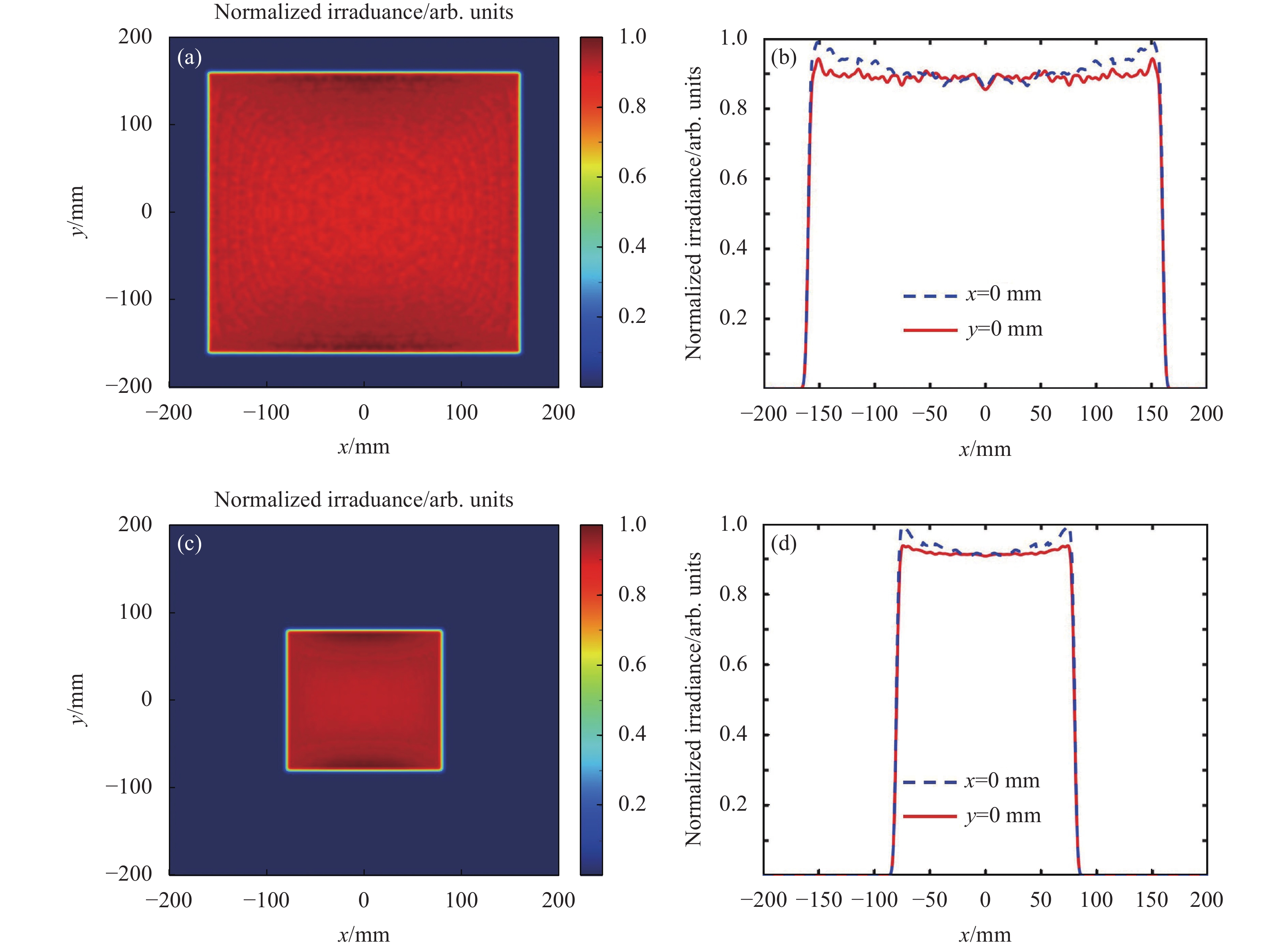
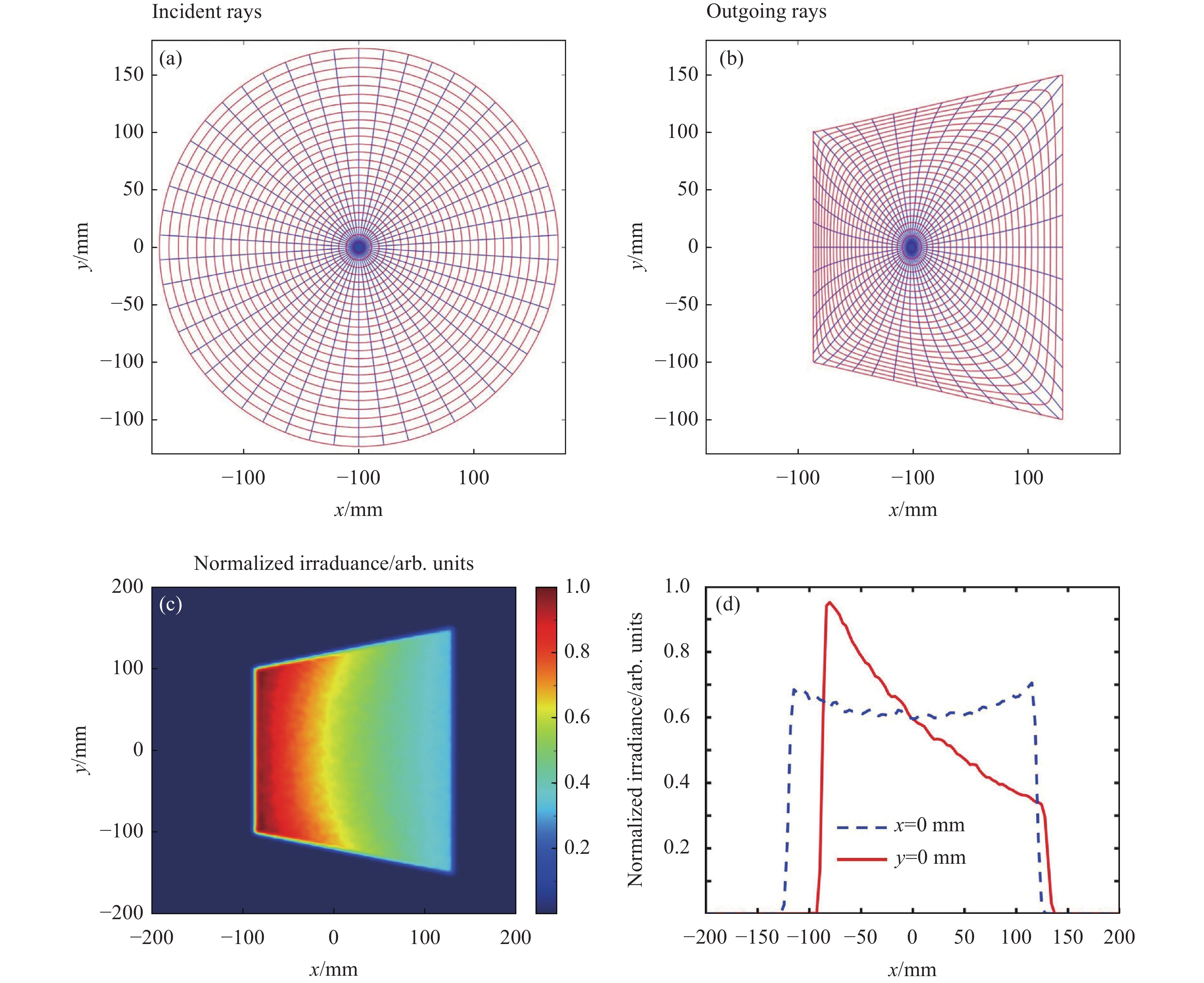
图6(a)给出了一组入射光线,其对应了光线不经过任何调控到达垂轴虚拟面上的光线落点分布,图6(b)则给出了入射光线经自由曲面透镜偏折后光线在垂轴虚拟面上的落点分布。从图6(b)中可知:经自由曲面透镜的偏折后,光线落点在垂轴面上呈梯形分布,并且梯形左侧光线密度大于右侧,这与图3(c)中的能量映射结果相对应。图6(a)和6(b)定义了经自由曲面透镜的调控后的光源和目标面落点之间的映射关系,这样不规则的映射分布展现了MA方程法在光束调控过程中的有效性。为进一步比较该透镜在目标倾斜面和垂轴虚拟面上的照明效果,将垂轴虚拟面作为能量接收面进行了光线追迹,仿真结果及归一化照度曲线分别如图6(c)和6(d)所示, 在该照明距离处的离轴目标面上的仿真结果如图4(a)所示。图6(c)和图4(a)进一步展示了同一个透镜在垂轴照明和离轴照明时所产生效果的差异性,也证实了针对离轴照明需求,对目标面的离轴特性进行分析的重要性,否则所得照明效果与预期相差甚远,且目标面离轴特性越明显,偏移越大。

图 6 垂轴虚拟面上的照明结果分析。(a)入射光束离散分布图;(b) MA方程求解得到的图(a)中光线到达垂轴虚拟面上的光线落点分布;(c) |SW|=300 mm处垂轴虚拟目标面上的仿真效果;(d)垂轴虚拟面上沿x=0 mm和y=0 mm的归一化照度曲线
Figure 6. Analysis of lighting results on the vertical virtual plane. (a) Discrete distribution of incident beam; (b) Ray drop points distribution on the vertical virtual plane obtained by solving the MA equation; (c) Simulation result on the vertical virtual plane when |SW|=300 mm; (d) Normalized irradiance curves along the lines x=0 mm and y=0 mm
-
非垂轴观测平面上自由曲面光束强度与波前调控是一项具有挑战性并值得探索的问题。文中在垂轴布局下自由曲面光束强度与波前调控的基础上,通过建立离轴光分布到垂轴光分布的映射变换,在倾斜光路布局下实现了对光束强度与波前的高效准确调控。该方法打破了垂轴光路布局的制约,获得了灵活的光路布局,对推动自由曲面光束调控的广泛应用有着积极作用。该方法仅采用两个自由曲面,便实现了对光束强度和波前两个属性的高效灵活调控,这将推动着光束调控系统向着功能全面化和系统紧凑化的方向发展。
Simultaneous modulation of beam intensity and wavefront with freeform surfaces on the off-axis target plane (invited)
-
摘要: 自由曲面光束强度与波前调控旨在借助多个自由曲面实现对光束强度与波前两个属性的精准调控,然而这一调控工作通常要求观测平面垂直于光轴,导致系统光路布局受限。针对这一问题,文中提出了一种可实现灵活光路布局的自由曲面光束强度与波前调控方法。首先设定一个垂直于光轴的虚拟观测平面,并建立目标离轴观测平面上的特定照明分布和该垂轴虚拟观测平面上相应照明分布之间的映射关系。结合斯涅耳定律、局部能量守恒定律和光程守恒约束,建立针对垂轴虚拟平面的带有非线性边界条件的光束调控Monge-Ampère (MA)方程,之后采用有限差分法求解该垂轴布局光束调控模型,进而得到非垂轴观测平面上自由曲面光束强度与波前调控的数值解。采用该方法设计了一个用于调控点光源光束强度与波前的自由曲面透镜,借助蒙特卡洛光线追迹,验证了该方法在非垂轴观测平面上自由曲面光束强度与波前调控中的有效性。
-
关键词:
- 自由曲面光束调控 /
- 强度及波前调控 /
- 离轴光学系统 /
- Monge-Ampère方程
Abstract:Objective Simultaneous modulation of beam intensity and wavefront with freeform surfaces is widely used in illumination optics and imaging optics. The current method of simultaneous modulation of beam intensity and wavefront is generally aimed at vertical-axis optical systems. However, the optical system generally has an off-axis layout to achieve a compact optical structure. In this paper, we proposed a method to design freeform surfaces to realize simultaneous modulation of beam intensity and wavefront on the tilted target plane. Methods Firstly, a virtual observation plane perpendicular to the optical axis is set up, and the mapping relationship between the specific irradiance distribution on the target off-axis observation plane and the corresponding irradiance distribution on the vertical axis virtual observation plane is established. Then the Monge–Ampère (MA) equation with nonlinear boundary conditions for the vertical virtual plane is established according to Snell's law, local energy conservation law, and optical path conservation constraints. Then the finite difference method is used to solve the beam control model of vertical axis layout, and the numerical solutions of beam intensity and wavefront modulation of freeform surface on the off-axis observation plane are obtained. Finally, the Monte Carlo ray tracing method is used to verify the effectiveness of the designed freeform surface. Results and Discussion The design example is to use two freeform surfaces to shape a Lambertian point source into a uniform square irradiance distribution on an off-axis target plane, the shaped beam is a divergent spherical wave, and the off-axis target surface has an inclination angle of 30 degrees. The obtained surfaces are intricate but smooth, continuous, and easy to fabricate. Researchers use 10 million rays for Monte Carlo tracing to verify the effectiveness of the designed lens. The irradiance distribution on the target plane demonstrates the effectiveness of the modulation of beam intensity, with the irradiance error RMS=0.0117. The analysis of the outgoing wavefront and the simulation results at different distances verify the effectiveness of the modulation of the beam wavefront. Conclusion Simultaneous modulation of beam intensity and wavefront is a challenging but worth exploring problem. In this paper, the efficient and accurate modulation of beam intensity and wavefront under an inclined optical path layout is realized by establishing the mapping transformation of off-axis irradiance distribution to vertical irradiance distribution. This method breaks the restriction of vertical optical path layout and obtains a flexible optical path layout, which plays an active role in promoting the wide application of freeform surface beam modulation. This method uses only two freeform surfaces to realize efficient and flexible modulation of beam intensity and wavefront, which will promote the beam control system towards the direction of comprehensive function and compact system. -
图 1 基于离轴目标面的自由曲面光束强度及波前调控模型
Figure 1. Model of beam intensity and wavefront control based on an off-axis target plane using freeform surfaces
图 2 离轴目标面到垂轴虚拟面的映射模型
Figure 2. Mapping model from off-axis target plane to vertical virtual plane
图 3 离轴面上光强和波前同时调控的设计实例。(a) 光束调控模型;(b)离轴目面上的目标照明分布;(c)映射为垂轴虚拟面上相应的照明分布;(d)入射面面型;(e)出射面面型;(f)自由曲面透镜模型
Figure 3. A design example of simultaneous control of light intensity and wavefront on off-axis plane. (a) Optical control model; (b) Target irradiance distribution of the off-axis target plane; (c) Mapping of the irradiance distribution on the vertical virtual plane; (d) Entrance surface; (e) Exit surface, and (f) the lens model
图 4 离轴目标面上照明效果的仿真验证。(a) |SW|=300 mm时倾斜目标面上的归一化照明分布;(b) |SW|=300 mm时沿着x=0 mm和y=0 mm的归一化照度曲线;(c)光程差分布
Figure 4. Simulation verification of lighting effects on the tilted target plane. (a) Normalized irradiance distribution on the tilted target plane of |SW|= 300 mm; (b) Normalized irradiance curves along the lines x=0 mm and y=0 mm; (c) Optical path difference distributions
图 5 不同照明距离处的仿真结果。(a) |SW|=400 mm时倾斜面上的照明分布;(b) |SW|=400 mm时沿着x=0 mm和y=0 mm的归一化照度曲线;(c) |SW|=200 mm时倾斜面上的照明分布;(d) |SW|=200 mm时沿着x=0 mm和y=0 mm的归一化照度曲线
Figure 5. Simulation results at different lighting distances. Normalized irradiance distribution on the tilted plane when |SW|=400 mm (a) and when |SW|=200 mm (c), normalized irradiance curves along the lines x=0 mm and y=0 mm when |SW|=400 mm (b) and when |SW|=200 mm (d)
图 6 垂轴虚拟面上的照明结果分析。(a)入射光束离散分布图;(b) MA方程求解得到的图(a)中光线到达垂轴虚拟面上的光线落点分布;(c) |SW|=300 mm处垂轴虚拟目标面上的仿真效果;(d)垂轴虚拟面上沿x=0 mm和y=0 mm的归一化照度曲线
Figure 6. Analysis of lighting results on the vertical virtual plane. (a) Discrete distribution of incident beam; (b) Ray drop points distribution on the vertical virtual plane obtained by solving the MA equation; (c) Simulation result on the vertical virtual plane when |SW|=300 mm; (d) Normalized irradiance curves along the lines x=0 mm and y=0 mm
-
[1] Reimers J, Bauer A, Thompson K P, et al. Freeform spectrometer enabling increased compactness [J]. Light: Science & Applications, 2017, 6(7): e17026. doi: https://doi.org/10.1038/lsa.2017.26 [2] Ge P, Li Y, Chen Z, et al. LED high-beam headlamp based on free-form microlenses [J]. Applied Optics, 2014, 53(24): 5570-5575. doi: 10.1364/AO.53.005570 [3] Zhu Z, Wei S, Liu R, et al. Freeform surface design for high-efficient LED low-beam headlamp lens [J]. Optics Communi-cations, 2020, 477: 126269. doi: https://doi.org/10.1016/j.optcom.2020.126269 [4] Ge P, Zhang K, Mao L, et al. An off-axis, reflective system for uniform near-field illumination in optical microscopy [J]. Ligh-ting Research & Technology, 2018, 50(5): 787-795. doi: https://doi.org/10.1177/147715351770700 [5] Taege Y, Schulz S L, Messerschmidt B, et al. A miniaturized illumination unit for airy light-sheet microscopy using 3D-printed freeform optics[C]//Imaging Systems and Applications, 2022. US: Optica Publishing Group, 2022: IW3C.1. [6] Yang L, Liu Y, Ding Z, et al. Design of freeform lenses for illuminating hard-to-reach areas through a light-guiding system [J]. Optics Express, 2020, 28(25): 38155-38168. doi: 10.1364/OE.411394 [7] Jin Y, Hassan A, Jiang Y. Freeform microlens array homogenizer for excimer laser beam shaping [J]. Optics Express, 2016, 24(22): 24846-24858. doi: 10.1364/OE.24.024846 [8] Feng Z, Froese B D, Liang R, et al. Simplified freeform optics design for complicated laser beam shaping [J]. Applied Optics, 2017, 56(33): 9308-9314. doi: 10.1364/AO.56.009308 [9] Mao X, Li J, Wang F, et al. Fast design method of the smooth freeform lens with an arbitrary aperture for collimated beam shaping [J]. Applied Optics, 2019, 58(10): 2512-2521. doi: 10.1364/AO.58.002512 [10] Yang T, Wang Y, Ni D, et al. Design of off-axis reflective imaging systems based on freeform holographic elements [J]. Optics Express, 2022, 30(11): 20117-20134. doi: 10.1364/OE.460351 [11] Wang Y, Yang T, Ni D, et al. Design of an off-axis near-eye AR display system based on a full-color freeform holographic optical element [J]. Optics Letters, 2023, 48(5): 1288-1291. doi: 10.1364/OL.484763 [12] Feng Z, Huang L, Gong M, et al. Beam shaping system design using double freeform optical surfaces [J]. Optics Express, 2013, 21(12): 14728-14735. doi: 10.1364/OE.21.014728 [13] Feng Z, Huang L, Jin G, et al. Designing double freeform optical surfaces for controlling both irradiance and wavefront [J]. Optics Express, 2013, 21(23): 28693-28701. doi: 10.1364/OE.21.028693 [14] Zhang Y, Wu R, Liu P, et al. Double freeform surfaces design for laser beam shaping with Monge-Ampère equation method [J]. Optics Communications, 2014, 331: 297-305. doi: https://doi.org/10.1016/j.optcom.2014.06.043 [15] Wei S, Zhu Z, Fan Z, et al. Double freeform surfaces design for beam shaping with non-planar wavefront using an integrable ray mapping method [J]. Optics Express, 2019, 27(19): 26757-26771. doi: 10.1364/OE.27.026757 [16] Doskolovich L L, Moiseev M A, Bezus E A, et al. On the use of the supporting quadric method in the problem of the light field eikonal calculation [J]. Optics Express, 2015, 23(15): 19605-19617. doi: 10.1364/OE.23.019605 [17] Bykov D A, Doskolovich L L, Byzov E V, et al. Supporting quadric method for designing refractive optical elements generating prescribed irradiance distributions and wavefronts [J]. Optics Express, 2021, 29(17): 26304-26318. doi: 10.1364/OE.432770 -

 点击查看大图

计量
- 文章访问数: 104
- HTML全文浏览量: 17
- PDF下载量: 42
- 被引次数: 0

