


 下载:
下载:


-
透过散射介质的成像在生物医学、水下探测等许多领域具有重要应用价值[1-5]。在众多散射成像技术中,基于光学记忆效应[6]和散斑相关的成像技术发展迅速。光学记忆效应包含了角度记忆效应和线性平移记忆效应。角度记忆效应指当光波的入射角度变化范围较小时,像面上所接收的散斑分布并不会随入射角度的改变而明显改变,仅产生一个与角度变化方向对应的整体位移,文中指角度记忆效应。Katz等提出了一种单帧散斑自相关(SSC)的非侵入式成像方法[7],这种方法利用高分辨率的单帧散斑图像的自相关性,使用相位迭代恢复算法对隐藏在散射介质后的目标成像[8],具有无需繁琐的标定过程,无需侵入散射系统内部等优点。单帧成像技术可缩短相机曝光时间,使得实时成像成为可能。在尽可能短的相机曝光时间内获得高质量的成像,需要消除影响成像质量的因素。SSC成像需要使用空间非相干光照明,以消除相干噪声对成像的影响。普通空间非相干光通常是宽频带光,宽带光会使得经过散射介质后形成的光学散斑对比度大大下降,从而无法利用散斑自相关来成像。频带窄的光如激光具有高的空间相干度,需要让光束通过旋转的散射片来获得空间非相干光。光束的空间相干性被消除的效果可由光斑对比度衡量,影响光斑对比度数值的三个主要因素是旋转散射片目数、转速和相机曝光时间,这三个因素对散斑相关成像质量的影响尚未见有研究报道。算法也是影响快速和高质量成像的重要因素。通常基于散斑相关的相位迭代恢复算法中需要对目标做多次初始随机猜测,从中遴选出恢复效果最好的图像,这需要耗费较长时间。如果已知散射系统的强度点扩展函数(PSF),则可用逆卷积运算重建隐藏目标[9]。已有用间接的方法得到系统的PSF的研究[10],这需要用一个已知的目标来测量PSF,也有用相位差法来恢复系统PSF的报道[11],这需要较高的实验技术。最好的方法是从未知目标的散斑图中直接提取散射系统的PSF,这将极有利于实际环境中的快速成像。最近,一种对目标域和系统光学传递函数加以约束的优化迭代算法被提出[12],这种方法能够在白光照明情况下重建隐藏在散射介质后的目标,同时给出系统的PSF信息。
综上所述,目前尚缺乏从实验系统的物理参数和算法角度对散斑相关快速成像进行系统性研究的工作。文中做了如下两方面的工作,第一是用旋转散射片生成空间非相干光束,分析了旋转散射片目数、转速和相机曝光时间对散斑相关成像的影响,给出了在不同的相机曝光时间下,为获取最好的成像效果应如何选择散射片转速。第二是将文献[12]的方法和散斑相关相位迭代算法结合,实现了在短的相机曝光时间下高质量快速成像,与只用散斑相关算法的情况相比成像质量显著提升。
-
SSC成像的物理基础是光学记忆效应[6]。照射目标的光束经过散射介质后出射的散斑光强可写为目标场$ O $与PSF之间的卷积:
$$ I\left( {{x'},{y'}} \right){\text{ = }}O\left( {x,y} \right)*h $$ (1) 式中:$ h $为PSF;*为卷积运算;$ \left( {{x'},{y'}} \right) $为像空间坐标;$ \left( {x,y} \right) $为物空间坐标。为重建目标,对散斑强度作自相关运算[7, 13]:
$$ I \otimes I = \left( {O * h} \right) \otimes \left( {O * h} \right) = \left( {O \otimes O} \right) * \left( {h \otimes h} \right) $$ (2) 式中:$ \otimes $为相关运算。窄频带照明光下,PSF的自相关$ h \otimes h $近似为一个尖锐的峰值$ \delta $函数,公式(2)可简化为:
$$ I \otimes I = \left( {O \otimes O} \right) * \delta \approx O \otimes O $$ (3) 利用散斑自相关可以得到隐藏目标的傅里叶振幅分布信息。对公式(3)作傅里叶变换可得:
$$ \begin{split} FT\left[ {I\left( {{x'},{y'}} \right) \otimes I\left( {{x'},{y'}} \right)} \right] =& FT\left[ {O\left( {x,y} \right) \otimes O\left( {x,y} \right)} \right]= \\ {\left| {FT\left[ {O\left( {x,y} \right)} \right]} \right|^2} =& {\left| {FT\left[ {I\left( {x,y} \right)} \right]} \right|^2} \end{split}$$ (4) 式中:$ FT $为傅里叶变换;$ |\cdots| $为求模运算。
公式(4)表明散斑强度分布自相关的傅里叶变换等于目标图像傅里叶幅值的平方,等式两边求均方根可得目标的傅里叶幅值分布:
$$ S({k_x},{k_y}) = |FT[O(x,y)]| = \sqrt {FT[I({x'},{y'}) \otimes I({x'},{y'})]} $$ (5) 因为目标信息集中在散斑图像自相关的中间部分,为提高图像重建效率,在计算的散斑自相关分布中增加窗口函数再进行傅里叶变换求解目标的傅里叶幅值信息:
$$ S({k_x},{k_y}) = \sqrt {\left| {FT\left[ {W(x,y)F{T^{-1}}\left\{ {{\text{|}}FT{\text{[}}I(x,y){\text{]}}{{\text{|}}^2}} \right\}} \right]} \right|} $$ (6) 窗函数$ W(x,y) $由被观察目标的大小来决定。基于SSC的相位迭代算法通常用于稀疏目标的散斑成像。最近用白光照明的散斑成像方法被提出[12]。此处作简单介绍,公式(1)在频域可写为[12]:
$$ FT(I)=FT(O)\cdot |FT(h)|{{\rm{e}}}^{i\theta } $$ (7) $ |FT(h)| $和$ {{\rm{e}}^{i\theta }} $代表点扩展函数的傅里叶变换的幅值和相位。对公式(7)作逆傅里叶变换可得:
$$ F{T}^{-1}\left[\frac{FT(I)}{{{\rm{e}}}^{i\theta }}\right]=O\ast F{T}^{-1}\left\{|FT(h)|\right\} $$ (8) 由Wiener-Khinchin定理,信号的功率谱可看作信号自相关的傅里叶变换。因此上式可进一步写为:
$$ F{T}^{-1}\left[\frac{FT(I)}{{{\rm{e}}}^{i\theta }}\right]=O\ast F{T}^{-1}\left[\sqrt{FT(h\otimes h)}\right] $$ (9) 其中,$ h \otimes h $即PSF的自相关可近似为一$ \delta $函数,因此公式(9)可近似写为:
$$ F{T}^{-1}\left[\frac{FT(I)}{{{\rm{e}}}^{i\theta }}\right]\approx O $$ (10) 重建目标从频域开始,初始对点扩展函数的相位${{\rm{e}}^{i\theta }}$做一随机猜测,利用上式进行迭代。第$ k $次迭代中目标的傅里叶谱可写为$FT({O}^{(k)})=FT(I)/{{\rm{e}}}^{i{\theta }^{(k)}}$,逆傅里叶变换回到目标域后需要对目标空间施加约束,更新目标$ {O^{(k)}} $后重复迭代直至较好的还原效果。迭代中点扩展函数的傅里叶谱可写为${A}^{(k)}{{\rm{e}}}^{i{\theta }^{(k)}}=FT(I)/FT({O}^{(k)})$,式中$ {A^{(k)}} $代表点扩展函数傅里叶谱的估算幅值,计算中可以用数字1替代$ {A^{(k)}} $作为对点扩展函数的一种频域约束。以上方法适用于窄频带光照明的散斑成像中恢复系统的PSF信息。窄频带光照明下如果透过散射介质后形成的光学散斑的对比度和信噪比不够高,直接用表达公式(7)~(10)得到的点扩展函数作解卷积运算重建目标得不到理想的还原效果。为解决以上问题,无需利用目标的先验信息,文中从一个任选的隐藏目标得到散射系统的点扩展函数,将该点扩展函数和SSC相位恢复算法相结合,实现了对不同大小、形状的目标的单次输入快速成像和高质量的重建效果。相比较只用SSC的相位恢复算法,文中给出的方法的成像速度和质量都显著提升。
-
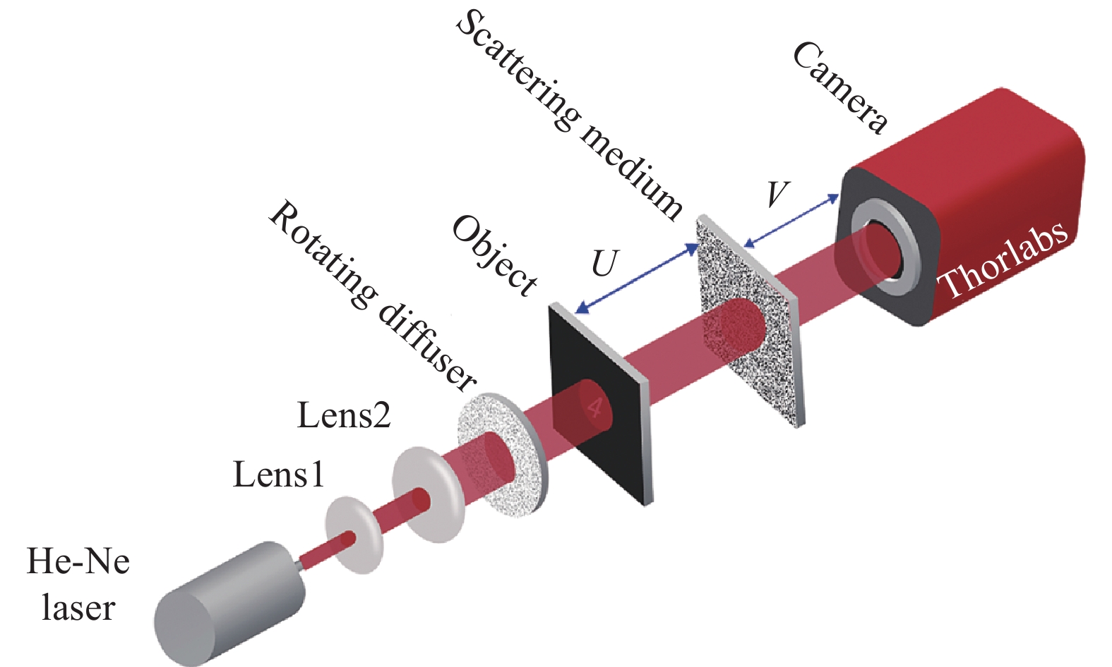
实验有两个目标,一是研究照射目标的光束的空间相干性对散斑相关成像质量的影响,二是研究成像算法对单帧散斑快速成像质量的影响。实验用He-Ne激光器(ThorLabs-HNL150LB, 632.8 nm)产生单色激光,自制旋转漫射器生成空间非相干的赝热光,旋转漫射器由直流电机驱动旋转的散射片组成,实验中研究了两种旋转散射片,即砂粒度为220目和600目(ThorLabs-DG20-220,DG20-600)的散射片生成空间非相干光的情况。实验装置如图1所示。
图1中rotating diffuser为旋转漫射器,CCD相机型号为ThorLabs-8051C。激光器发出的光束经过旋转漫射器后生成空间非相干光,照射目标后透过散射介质生成的光学散斑由相机拍摄。散射介质是砂粒度为600目的散射片(ThorLabs-DG10-600)。在第一步研究光束的空间相干性对成像质量影响的研究中,空间非相干光的生成效果可由光斑对比度分析,这时将相机直接放在旋转漫射器后拍摄光斑图像。
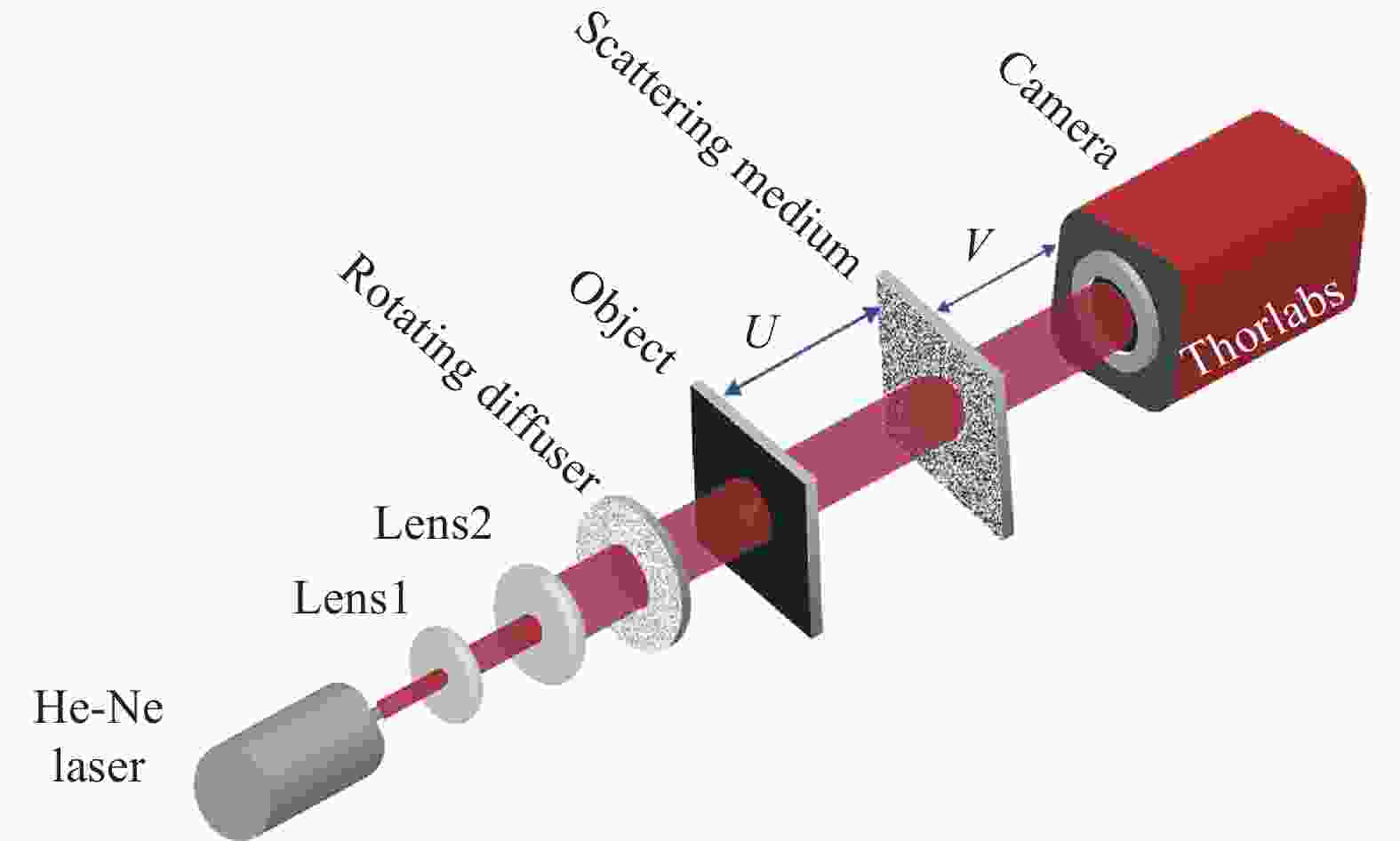
图 1 散斑成像实验装置图
Figure 1. Experimental setup for scattering imaging
-
如图1所示实验装置,激光光束通过旋转漫射器后生成空间非相干光照射目标。光束通过旋转散射片后消除空间相干性的原理如图2所示,散射片在x-y平面内沿顺时针方向旋转,光束传播方向垂直于x-y平面。
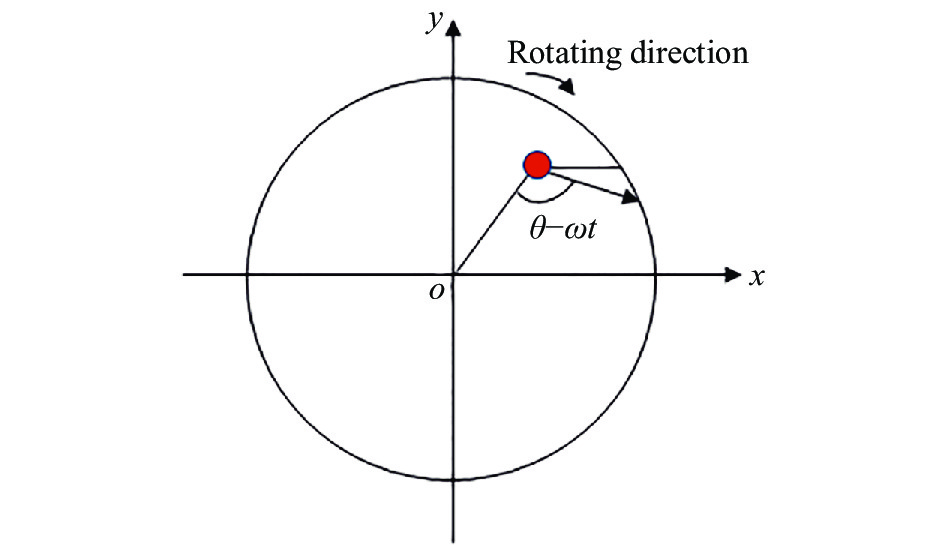
图 2 散射片旋转示意图
Figure 2. Schematic diagram of rotation of diffuser
光经过旋转散射片后出射面上每个点的光相位在一定范围内随时间随机变化,这减少了散斑场的相干时间,在CCD相机的一个积分时间内接收的不相关散斑场的个数增加,这些不相关散斑场的叠加可抑制相干散斑噪声。光束空间相干性被消除的效果受旋转散射片目数、转速和相机曝光时间的影响。光斑对比度可衡量光束空间相干性被消除的效果,公式为[14]:
$$ C = \frac{\sigma }{{\left\langle I \right\rangle }} $$ (11) 式中:$ \sigma $为光强的标准差;$ \left\langle I \right\rangle $为光强的平均。图3是相机采集的光斑图,显示了光斑对比度随散射片转速的变化。转速的单位$\; {\rm{r}}/{\rm{s}}$表示转每秒,即每秒钟所转的圈数。
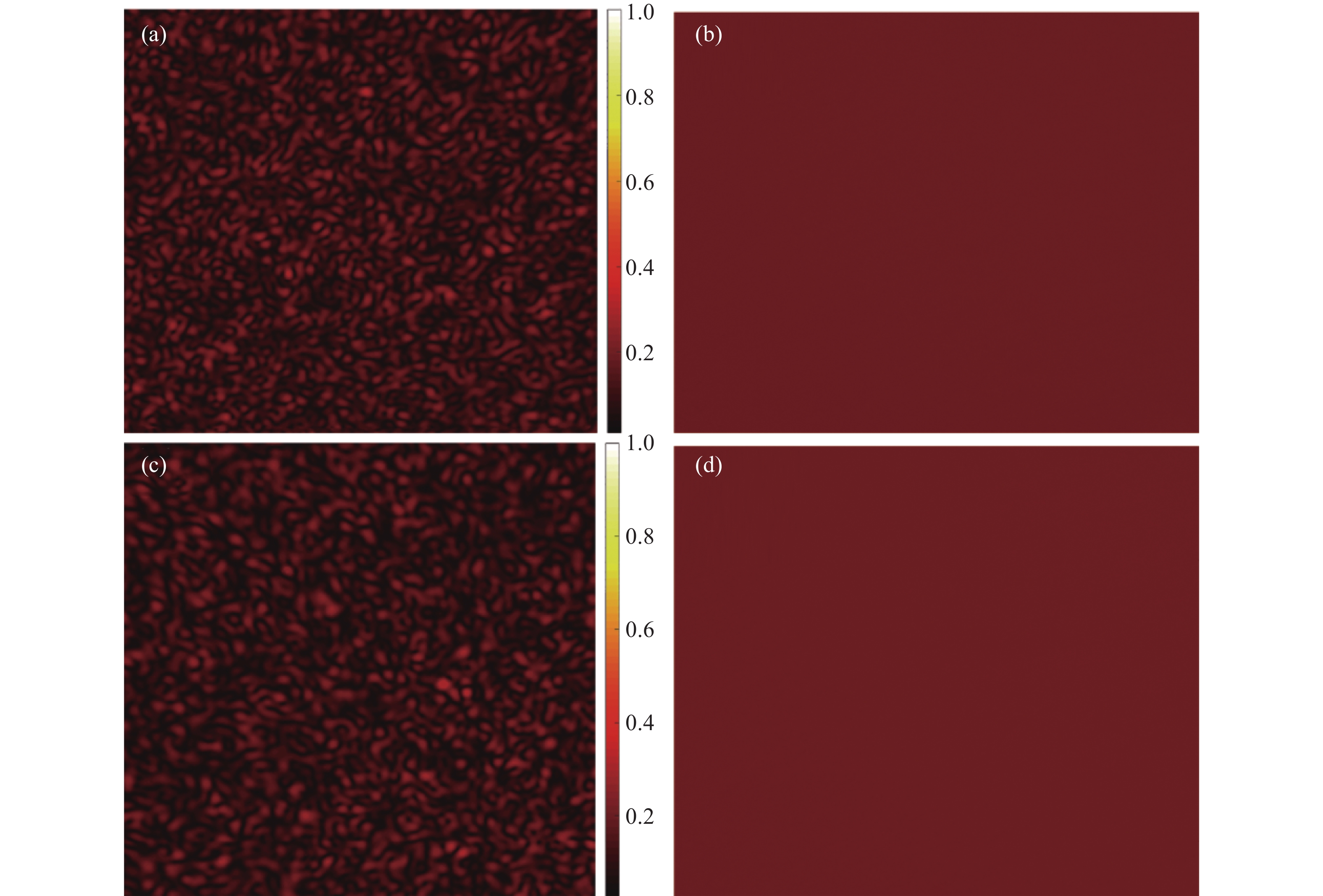
图3(a)、(c)为散射片静止时采集的散斑图,图3(a)显示220目散射片$0\;\; {\rm{r}}/{\rm{s}}$时的情况,对比度为$ C{\text{ = }}0.43 $,这是典型的散斑对比度值[15]。图3(c)显示600目散射片$0 \; {\rm{r}}/{\rm{s}}$时的情况,对比度为$ C{\text{ = }}0.403\;5 $。图3(b)、(d)为旋转散射片$80 \; {\rm{r}}/{\rm{s}}$时采集的光斑图,图3(b)显示220目散射片$80 \; {\rm{r}}/{\rm{s}}$时的情况,对比度为$ C = 0.007\;45 $,图3(d)显示600目散射片$80 \; {\rm{r}}/{\rm{s}}$时的情况,对比度为$ C{\text{ = }}0.007\;1 $。图3表明220目和600目旋转散射片均能使散斑对比度大大降低,光斑变得均匀,生成空间非相干光束。
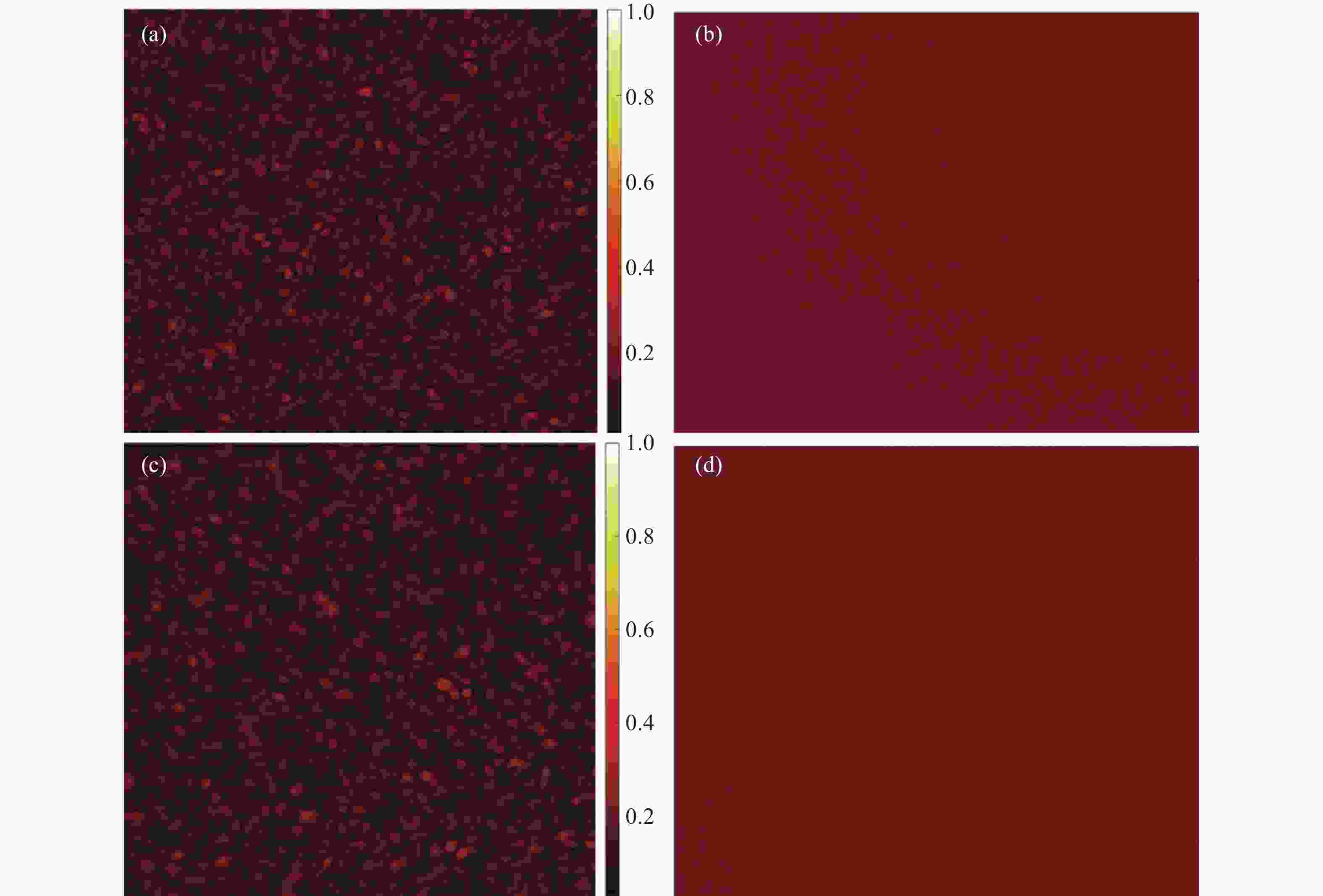
图 3 散斑图光斑对比度随散射片转速的变化。相机曝光时间为160 ms,颜色条代表光强相对值。(a)旋转散射片为220目,转速为0 r/s;(b) 转散射片为 220目,转速为80 r/s; (c)旋转散射片为600目,转速为0 r/s;(d) 旋转散射片为 600目,转速为80 r/s
Figure 3. Speckle contrast of the speckle pattern versus the rotational rate of diffuser. The exposure time of camera is 160 ms. The color bar represents the relative value of light intensity. (a) The cases of 220 grit ground glass diffuser. The rotational rate is 0 r/s; (b) The cases of 220 grit ground glass diffuser. The rotational rate is 80 r/s; (c) The cases of 600 grit ground glass diffuser. The rotational rate is 0 r/s; (d) The cases of 600 grit ground glass diffuser. The rotational rate is 80 r/s
-
光束通过旋转漫射器后生成空间非相干光束,照射目标后透过散射介质形成光学散斑。相机接收的散斑可由SSC的相位恢复算法重建目标图像。影响成像质量的因素包含了旋转散射片目数、转速和相机曝光时间。成像质量则可用相关系数分析,这里相关系数指的是SSC成像图像和目标原图之间的相关系数,计算式如下:
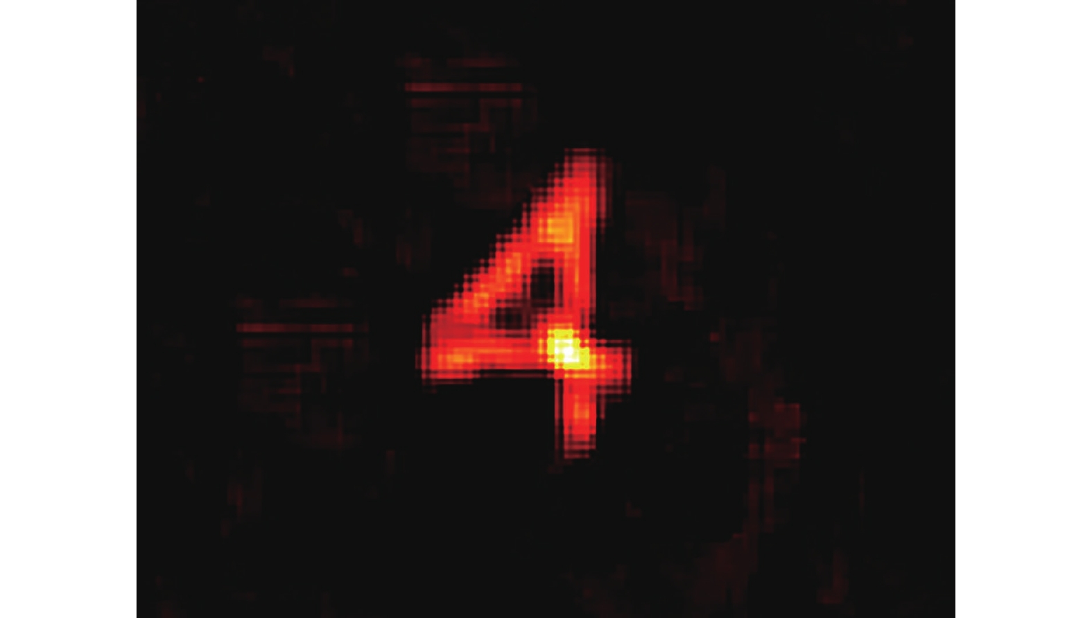
$$ Corr = \frac{{\displaystyle\sum\limits_m {\displaystyle\sum\limits_m {({A_{mn}} - \overline A )({B_{mn}} - \overline B )} } }}{{\sqrt {\left( {\displaystyle\sum\limits_m {\displaystyle\sum\limits_m {{{({A_{mn}} - \overline A )}^2}} } } \right)\left( {\displaystyle\sum\limits_m {\displaystyle\sum\limits_m {{{({B_{mn}} - \overline B )}^2}} } } \right)} }} $$ (12) 式中:$ {A_{mn}} $和$ {B_{mn}} $分别代表成像图和目标原图的像素强度值;$ \overline A $和$ \overline B $分别代表两图像素强度的平均值。实验中旋转漫射器使用220目散射片,散射介质是600目的散射片(ThorLabs-DG10-600)。本节中的成像目标为定制的负片“4”字,大小$73\;{\text{μ}} {\rm{m}} \times 104\;{\text{μ}} {\rm{m}}$。图4是用SSC相位恢复算法重建的图像,相机曝光时间为$100\; {\rm{ms}}$,旋转散射片为$80 \; {\rm{r}}/{\rm{s}}$。

图 4 旋转散射片80 r/s时目标的散斑相关成像
Figure 4. Speckle correlation imaging when the rotational rate of diffuser is 80 r/s
图4显示旋转散射片在$ 80 \; {\rm{r}}/{\rm{s}} $时成像相关系数为$ Corr = 0.834\;5 $。旋转漫射器目数、转速和相机曝光时间对散斑相关成像的影响在图5中进一步分析。
图5显示光斑对比度及成像相关系数随旋转漫射器散射片转速的变化。其中成像相关系数指用SSC相位恢复算法重建的图像与目标原图之间的相关系数。图(a)~(d)显示220目旋转散射片的情况,图(e)~(h)显示600目旋转散射片的情况,图(a)~(f)显示旋转漫射器转速变化时光斑对比度的变化, 图(c)~(h) 显示旋转漫射器转速变化时成像相关系数的变化。 旋转散射片转速从$ 10 \; {\rm{r}}/{\rm{s}} $增加到$ 100 \; {\rm{r}}/{\rm{s}} $,每次增加$ 10 \; {\rm{r}}/{\rm{s}} $。从图5可总结如下:1) 随旋转漫射器散射片转速和相机曝光时间的增加,光斑对比度下降,成像相关系数上升。相机曝光时间为$ 40\; {\rm{ms}} $时,光斑对比度和成像相关系数随散射片转速变化较大,转速$ 10 \; {\rm{r}}/{\rm{s}} $时对比度为0.017,转速$ 100 \; {\rm{r}}/{\rm{s}} $时对比度为0.01545,大约下降了9%。转速$10\; {\rm{r}}/{\rm{s}}$时成像相关系数为0.6403,转速$ 90 \; {\rm{r}}/{\rm{s}} $时成像相关系数为0.7304,成像相关系数提升约14%。转速$ 80 \; {\rm{r}}/{\rm{s}} $时,$ 220\; {\rm{ms}} $曝光时间下的成像相关系数相比$ 40\; {\rm{ms}} $曝光时间下的成像相关系数提升约21%。当旋转散射片转速超过$ 100 \; {\rm{r}}/{\rm{s}} $时,机械振动等因素使得重建图像中噪声增加, 成像相关系数有所下降。2) 相机曝光时间超过$ 100\; {\rm{ms}} $后,光斑对比度和成像相关系数随散射片转速的变化相对较小,变化小于10%。3) 旋转散射片砂粒度为600目的情况相比220目的情况,光斑对比度下降。如曝光时间为$ 40\; {\rm{ms}} $和散射片转速为$ 80 \; {\rm{r}}/{\rm{s}} $时,220目旋转散射片对应的光斑对比度为0.01615和成像相关系数为0.717,600目旋转散射片对应的光斑对比度为0.0146和成像相关系数为0.735,成像质量有小幅度改善。4) 同一散射片转速下,随着相机曝光时间的增加,光斑对比度和成像相关系数呈非线性变化。图6显示了散射片转速为$ 80 \; {\rm{r}}/{\rm{s}} $的情况。
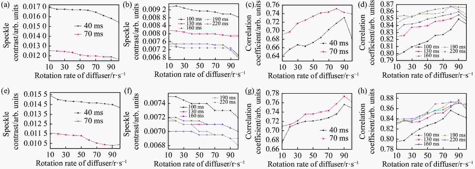
图 5 光斑对比度及成像相关系数随散射片转速的变化。(a)~(d)显示220目旋转散射片的情况,(e)~(h)显示600目旋转散射片的情况;(a)、(c)、(e)、(g)显示相机曝光时间为40 ms和70 ms的情况,(b)、(d)、(f)、(h)显示相机曝光时间为100 ms、130 ms、160 ms、190 ms、220 ms的情况;(a)、(b)、(e)、(f)光斑对比度随旋转散射片转速的变化,(c)、(d)、(g)、(h)目标“4”成像相关系数随旋转散射片转速的变化
Figure 5. Speckle contrast and imaging correlation coefficient versus the rotational rate of diffuser. The cases of the 220 grit rotation diffuser are shown in (a)-(d), the cases of the 600 grit rotation diffuser are shown in (e)-(h); The exposure time of camera is 40 ms and 70 ms in (a), (c), (e) and (g), the exposure time of camera is 100 ms, 130 ms, 160 ms, 190 ms and 220 ms in (b), (d), (f) and (h); The cases of the speckle contrast versus the rotational rate of rotating diffuser are shown in (a), (b), (e) and (f), correlation coefficient of speckle correlation imaging of target "4" versus rotation rate of diffuser are shown in (c), (d), (g) and (h)
图6显示光斑对比度和成像相关系数随相机曝光时间的变化。旋转散射片砂粒度为220目,转速固定为$ 80 \; {\rm{r}}/{\rm{s}} $。当曝光时间小于$ 100\; {\rm{ms}} $时,光斑对比度和成像相关系数随相机曝光时间的变化较大,大致成线性。 曝光时间超过$ 100\; {\rm{ms}} $后,光斑对比度和成像相关系数随相机曝光时间的变化较小,曲线变得平缓。这显示小于$ 100\; {\rm{ms}} $的相机曝光时间内,非相关散斑场的叠加不足以导致散斑的不均匀性被完全消除,光斑对比度和成像相关系数会随相机曝光时间的增加而变化较大。曝光时间超过$ 100\; {\rm{ms}} $后非相关散斑场的叠加使得光斑变得较为均匀,光斑对比度和成像相关系数随相机曝光时间的变化很小。 这些研究对于不同曝光时间的单帧散斑相关成像均有重要意义。对于曝光时间短的快速成像,较高的漫射器转速相比低转速可以较大幅度地提升成像质量,但转速过高引入的机械噪声也可能导致成像质量下降。对于相对长的相机曝光时间,漫射器转速的变化对于散斑相关成像质量的影响较小。

图 6 光斑对比度及成像相关系数随曝光时间的变化(散片转速为80 r/s)。(a)散斑对比度随曝光时间的变化;(b)成像相关系数随曝光时间的变化
Figure 6. Speckle contrast and imaging correlation coefficient versus the exposure time (The rotational rate of diffuser is 80 r/s). (a) Speckle contrast versus the exposure time; (b) Correlation coefficient versus the exposure time
-
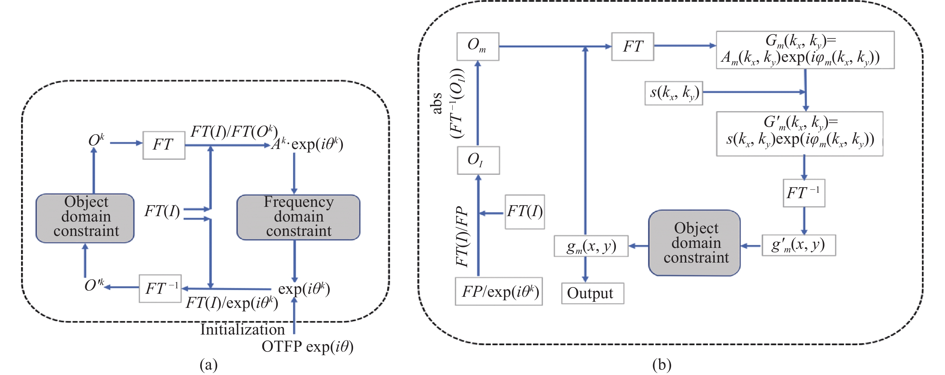
高质量的单帧散斑快速成像需要重建算法尽可能压缩运行时间,同时尽可能提高成像质量。通常基于SSC的HIO-ER相位恢复算法需要对目标作初始的随机猜测后迭代恢复[8],为得到好的重建效果,目标图像的初始猜测往往需要循环许多次。文中提出了一种将系统PSF和SSC相位恢复算法结合来避免目标的初始随机猜测的方法。系统PSF的提取无需实验目标的先验信息,直接从目标散斑获得。与只用SSC相位恢复算法相比,该方法显著提升了成像质量和压缩了图像重建时间。算法示意图如下:
上图中$ OTFP $代表对点扩展函数作傅里叶变换后的频谱相位。$ FP $代表散射系统的PSF的频谱相位,$ FT(I) $代表目标的散斑强度图像的傅里叶变换。图7(a)中使用了对未知实验目标的目标域约束和PSF的频域约束,迭代得到系统的PSF信息。初始对PSF的傅里叶相位作随机猜测,根据目标恢复效果$ {O^{(k)}} $确定散射系统的PSF。求出的系统PSF适用于不同大小、不同形状的目标,即对不同的成像目标,如位置变化范围较小,则无需再求PSF,直接使用图7(a)中散射系统PSF即可。图7(b)中$ FP $是系统PSF的频谱相位,即图7(a)中得到的系统PSF的频谱相位,对确定的散射系统,$ FP $是确定的,不随成像目标而变。利用公式${O_m} = abs\left\{ {F{T^{-1}}\left[ {FT(I)/FP} \right]} \right\}$得到重建目标的初始图像,其中$ F{T^{-1}} $是逆傅里叶变换。将此初始图像代入HIO-ER相位恢复算法中重建目标。图7中(a)和(b)部分的目标域约束是不一样的,(a)中为非零像素约束法(NNP)[16],(b)中为HIO-ER算法[8],如下:
$$ HIO算法: {g_m}\left( {x,y} \right) = \left\{ {\begin{array}{*{20}{c}} {{g_m}'\left( {x,y} \right)}&{\left( {x,y} \right) \in M} \\ {{g_m}\left( {x,y} \right) - \beta {g_m}'\left( {x,y} \right)}&{\left( {x,y} \right) \notin M} \end{array}} \right. $$ $$ ER算法: {g_m}\left( {x,y} \right) = \left\{ {\begin{array}{*{20}{c}} {{g_m}'\left( {x,y} \right)}&{\left( {x,y} \right) \in M} \\ 0&{\left( {x,y} \right) \notin M} \end{array}} \right. $$ 式中:$ M $表示函数$ {g_m}'\left( {x,y} \right) $满足实空间约束的元素集合。下文将图7(b)算法简写为PSF+HIO。
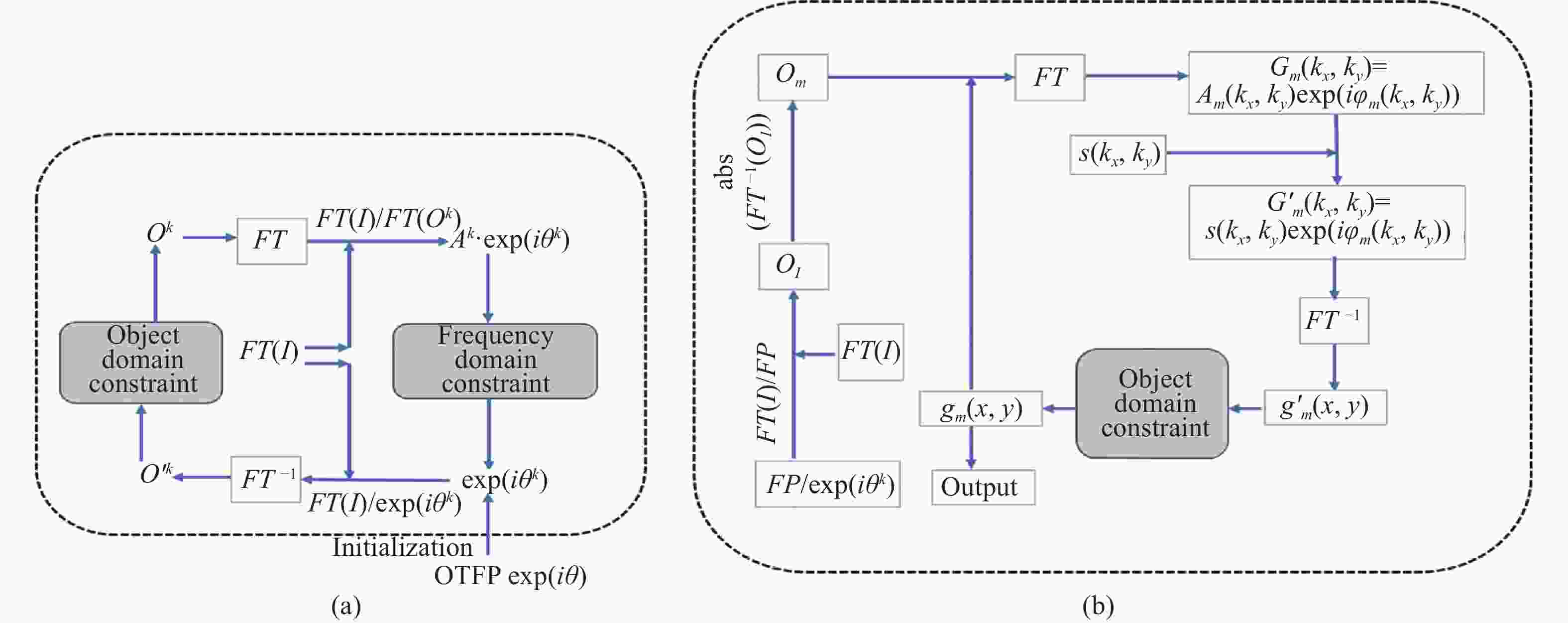
图 7 相位恢复算法框图 。(a)获取初始目标的PSF;(b) PSF与HIO&ER混合算法
Figure 7. Schematic of phase retrieval algorithm. (a) Obtaining PSF of initial target; (b) Scheme of PSF and HIO&ER hybrid algorithm
-
已有文献研究了用散斑差值自相关[17]和瞬时散斑多路复用[18]对运动目标的实时追踪和视频成像,以及用散射介质的傅里叶域浴帘效应和相干衍射迭代恢复算法实现散射介质后的超分辨成像[19],但尚未见有短曝光时间下同时提高单帧散斑的成像质量与速度的研究。笔者分析了相机曝光时间分别为$ 40\; {\rm{ms}} $和$ 160\; {\rm{ms}} $两种情况,由2.2节实验结果,将漫射器转速设为$ 80 \; {\rm{r}}/{\rm{s}} $。算法如上节所示。
实验装置见图1,旋转散射片砂粒度为600目(ThorLabs-DG20-600)。散射介质是600目的散射片(ThorLabs-DG10-600)。实验目标“4”成像时目标到散射介质距离$ u = 3\; {\rm{cm}} $和散射介质到相机距离$ v = 4\;{\rm{cm}} $。目标为三个数字负片,依次为“4”、“2”、“3”,大小相应为$73 \;{\text{μ}}{\rm{m}} \times 104\;{\text{μ}}{\rm{m}}$、$114\;{\text{μ}}{\rm{m}} \times 178\;{\text{μ}}{\rm{m}}$、$113 \;{\text{μ}}{\rm{m}}\times 178\;{\text{μ}}{\rm{m}}$。
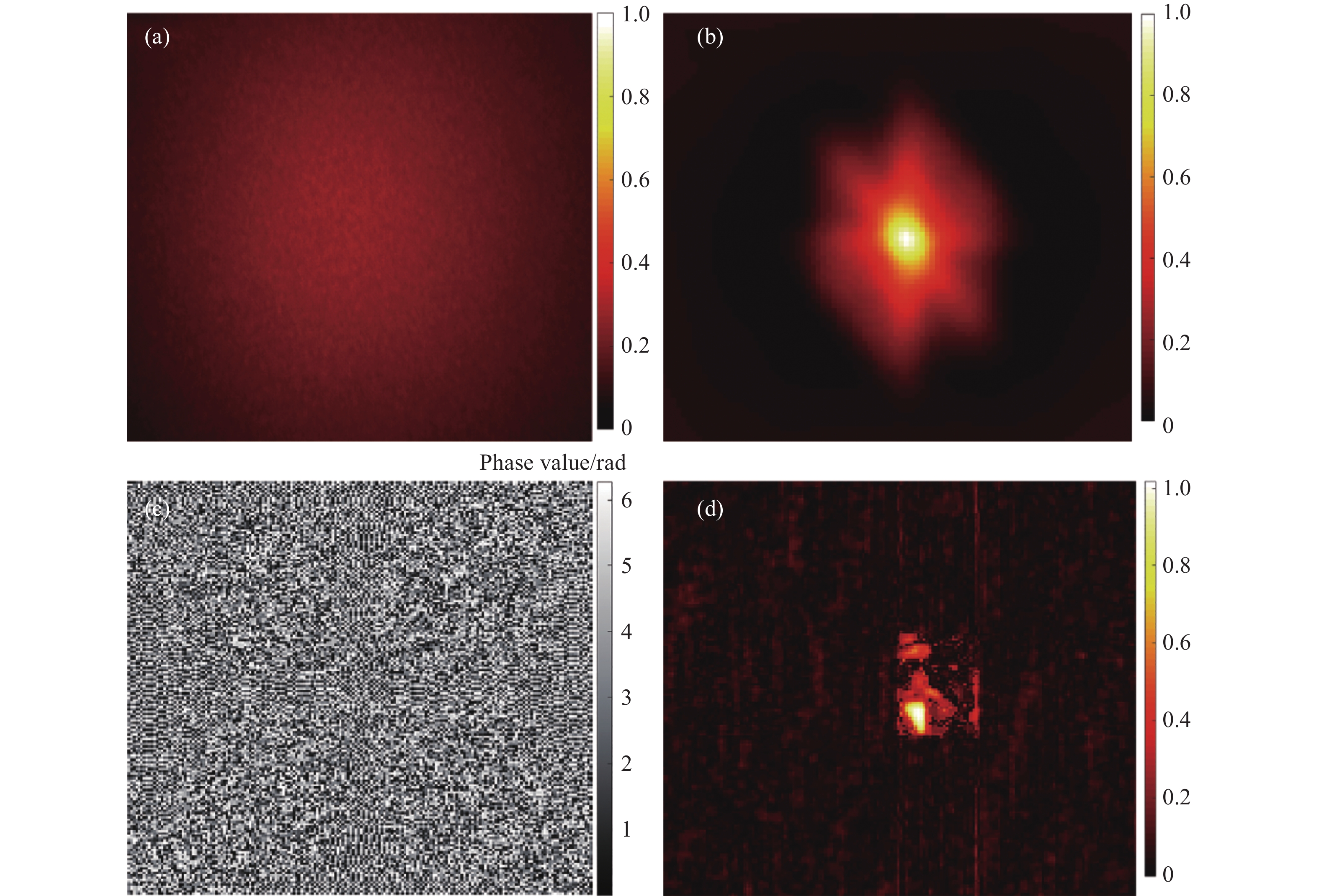
图8是显微镜下目标“4”、目标“2”、目标“3”的原图。图9是用实验目标“4”得到散射系统PSF的结果,相机曝光时间为$ 160\; {\rm{ms}} $。相机曝光时间$ 40\; {\rm{ms}} $成像时也使用该PSF。图9(a)显示目标“4”的光学散斑。图9(b)为单帧散斑的自相关运算,在NNP约束中需选取自相关区域作为约束区域。图9(c)显示PSF的傅里叶相位,PSF获得方法如图7(a)所示。图9(d)显示用PSF解卷积得到的目标初始图像。

图 8 显微镜下目标原图。(a)目标“4”;(b) 目标“2”;(c) 目标“3”
Figure 8. Original image of target by microscope. (a) Target “4”; (b) Target “2”; (c) Target “3”

图 9 目标“4”实验结果,颜色条显示光强的相对值。(a)光学散斑;(b) 自相关;(c) PSF傅里叶相位;(d) PSF解卷积恢复目标
Figure 9. Experimental results of target “4”. The color bar represents the relative value of the light intensity. (a) Optical Speckle; (b) Speckle autocorrelation; (c) Fourier phase of PSF; (d) Image of target by PSF deconvolution
从图9(d)可知,用PSF解卷积恢复的目标图像未达到理想效果。这里使用PSF+HIO算法,即将PSF解卷积得到的目标初始图像代入SSC相位恢复算法中恢复目标。在HIO-ER相位恢复算法中,首先使用HIO算法,${\beta}$以0.04的步长从2逐步下降为0,每一步迭代30次,然后将HIO算法得到的结果作为初始值代入ER算法中继续迭代30次,得到最终成像结果。迭代次数超过30次对成像质量的提升影响很小,会延长成像时间。在Inteli7-10700F芯片的台式机上,在Matlab2018b中PSF+HIO算法的成像运行时间为4.5 s。图10显示用PSF+HIO算法对不同大小和形状目标的成像效果,并与只使用SSC相位恢复算法的成像效果进行了对比,相机曝光时间为$ 40\; {\rm{ms}} $。
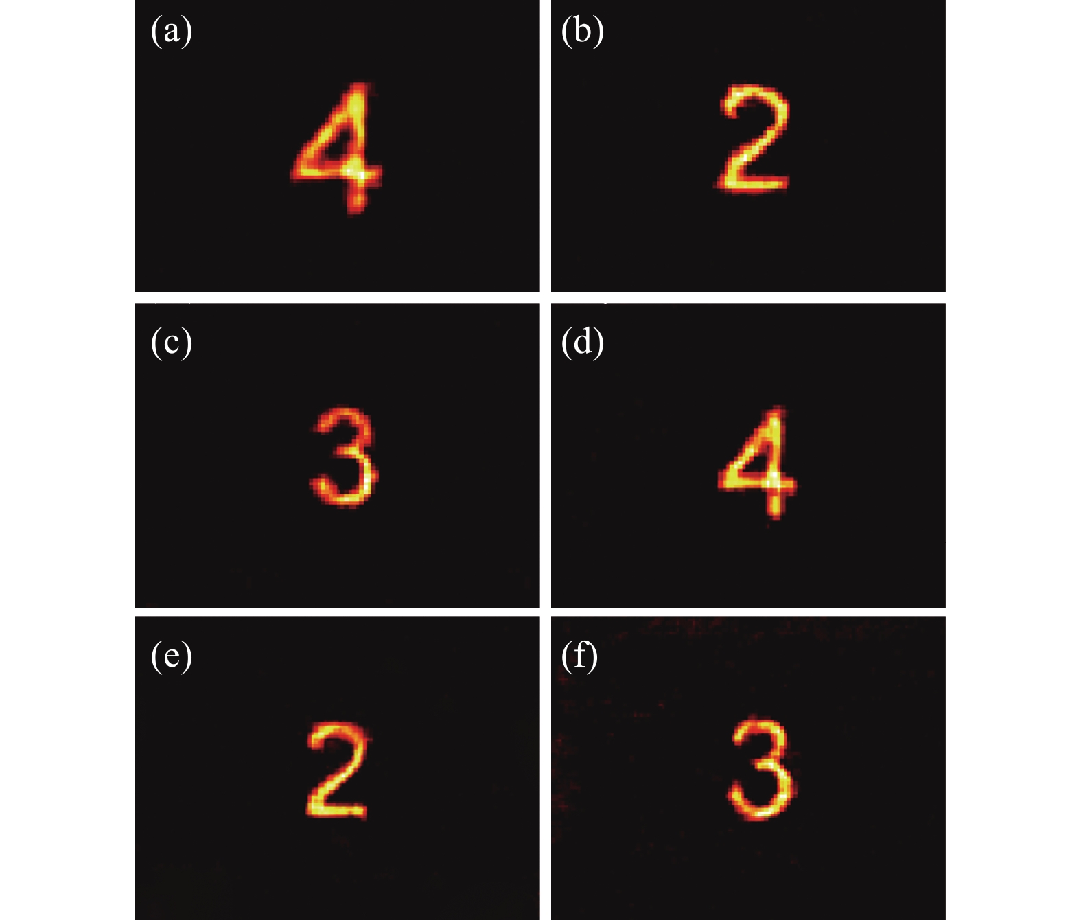
图10实验中用目标“4”得到系统的PSF。利用PSF+HIO算法恢复了目标“4”、“2”和“3”,并与只使用HIO相位算法的成像结果进行对比。图10(a)~(c)使用PSF+HIO算法,图10(d)~(f)用HIO相位算法。图10(a)~(c)的成像相关系数分别为0.887 2、0.890 8和0.872 8, 图10(d)~(f)为0.717、0.736 4和0.75。图10显示, PSF+HIO算法相比只使用HIO相位算法可使成像质量大幅提升。PSF+HIO算法另一优势体现在成像速度。只使用HIO相位算法成像时需要对目标的初始图像作多次随机猜测,人为选择最优的结果,PSF+HIO算法免去了对目标的初始随机猜测,PSF输入算法即可一次成像,成像时间大为缩短。为全面了解算法性质,在$ 160\; {\rm{ms}} $相机曝光时间下对比了成像效果。

图 10 40 ms下成像重建结果。(a)~(c)使用PSF+HIO算法;(d)~(f)中只用SSC相位恢复算法
Figure 10. Reconstruction image under 40 ms. The PSF+HIO algorithm is used to reconstruct images in (a)-(c). The speckle autocorrelation algorithm is used to reconstruct images in (d)-(f)
图11的相机曝光时间是$ 160\; {\rm{ms}} $。图11(a)~(c)使用PSF+HIO算法,图11(d)~(f)用HIO相位算法。图11(a)~(c)的成像相关系数分别为0.904 2、0.889 2和0.890 9,图11(d)~(f)为0.85、0.826 9和0.858。图10与图11对比可知,使用PSF+HIO算法,相机曝光时间$ 40\; {\rm{ms}} $和$ 160\; {\rm{ms}} $下图像的成像质量相差较小,原因是使用系统PSF得到目标初始图像后,将该初始图像代入至SSC相位恢复算法中通过迭代运算逼近了目标原图。$ 160\; {\rm{ms}} $曝光时间下,PSF+HIO算法的成像质量和只用SSC相位恢复算法的成像质量相比差异较小。

图 11 160 ms下成像重建结果。(a)~(c)使用PSF+HIO算法;(d)~(f)中只用SSC相位恢复算法
Figure 11. Reconstruction image under 160 ms. The PSF+HIO algorithm is used to reconstruct images in (a)-(c). The speckle autocorrelation algorithm is used to reconstruct images in (d)-(f)
-
实验研究了单帧散斑自相关成像中空间非相干赝热光的生成以及对成像质量的影响。自制旋转漫射器生成空间非相干光,研究了旋转散射片转速、目数、相机曝光时间对生成光斑的对比度以及成像质量的影响。发现如下:1)旋转漫射器转速增加和CCD相机曝光时间增加都会使得散斑对比度下降,成像相关系数上升,当CCD相机曝光时间超过$ 100\; {\rm{ms}} $后,光斑对比度和成像相关系数随曝光时间和散射片转速的变化较小。2)旋转散射片目数由220增加到600时,生成光斑的对比度小幅下降,成像相关系数小幅上升。3)过高的散射片转速也容易引入机械振动等噪声,从而影响散斑相关成像质量。短相机曝光时间下的单帧散斑相关快速成像,选择最合适的散射片转速对获取高质量的成像结果非常重要。
利用对系统点扩展函数施以频域约束和目标域施以非零像素约束的迭代算法,无需实验目标的先验信息可恢复系统强度点扩展函数,结合单帧散斑自相关算法实现了对不同大小和形状的目标的高质量快速成像。在短至$ 40\; {\rm{ms}} $的相机曝光时间下,该方法在成像速度和成像质量上都显著优于只使用单帧散斑自相关的算法。该方法也能使$ 40\; {\rm{ms}} $曝光时间下的成像质量接近$ 160\; {\rm{ms}} $曝光时间下的成像质量。这对于高质量的单帧散斑快速成像乃至动态成像具有意义。
High quality and rapid imaging of single-shot optical speckle
-
摘要: 利用基于光学记忆效应的单帧散斑自相关方法,研究了光透过随机散射介质的快速成像。短的相机曝光时间内的高质量快速成像需要尽可能消除影响成像质量的因素。通过引入旋转散射片来消除光束的空间相干性,避免相干噪声对成像质量的影响。光斑对比度可衡量光束的空间相干性被消除的效果,影响光斑对比度数值的主要因素有三个:旋转散射片介质颗粒度即目数、转速、相机曝光时间。实验分析了220目数和600目数两种旋转散射片和不同转速、相机不同曝光时间的情况。结果表明,转速提高和相机曝光时间的增加均使得光斑对比度下降并提升散斑相关成像质量,相机曝光时间超过一定值后,光斑对比度和成像相关系数随散射片转速和曝光时间的变化相对较小。因此对于相机曝光时间短的单帧散斑快速成像,选择最合适的散射片转速对高质量成像非常重要。通过优化算法来提升成像质量。根据对光学传递函数约束的迭代算法,无需利用目标的先验信息即可恢复系统的点扩展函数,该点扩展函数适用于不同形状、不同大小的目标,结合单帧散斑自相关算法可实现快速成像,与仅使用单帧散斑自相关算法的情况相比成像质量显著提升。Abstract:
Objective The pursuit of high-quality optical rapid imaging through scattering media is crucial for real-time and dynamic imaging applications. The primary focus is on achieving excellent imaging quality within a short camera exposure time, necessitating the identification and mitigation of factors that degrade optical rapid imaging. In this study, the single-shot speckle autocorrelation method, leveraging the optical memory effect, is employed to investigate optical rapid imaging through scattering media. To address the challenge of spatial coherence in laser beams, a rotating diffuser is introduced. This diffuser effectively eliminates spatial coherence, thus preventing the adverse impact of coherent noise on imaging quality. The speckle contrast serves as a metric to quantify the effectiveness of spatial coherence elimination. Parameters such as grain size, rotation rate of the diffuser, and camera exposure time are examined for their influence on speckle contrast. Furthermore, the study emphasizes the significance of optimizing imaging algorithms to enhance the quality of rapid imaging. A systematic exploration of experimental factors and imaging algorithms contributes to the overall understanding and improvement of high-quality optical rapid imaging through scattering medium. Methods A rotating diffuser is introduced to eliminate the spatial coherence of the laser beam, so the impact of coherent noise on imaging quality is avoided. The speckle contrast can be used to measure the effect of eliminating the spatial coherence of the beam. For investigating the impact of rotating diffusers on the quality of optical rapid imaging, different cases involving 220-grit and 600-grit rotating diffusers, various rotational rates, and different camera exposure times are analyzed. The rotational rate of the diffuser ranges from 10 to 100 revolutions per second, increasing in increments of 10 revolutions per second. The camera exposure time is varied from 30 to 220 milliseconds, increasing in increments of 30 milliseconds. The study examines the speckle contrast and imaging correlation coefficient concerning the rotational rate of the diffuser and the camera exposure time (see Fig.5). To restore the point spread function of the system without relying on prior information of the target, an iterative optimization algorithm for the optical transfer function constraint is employed. The imaging algorithm, combining the point spread function with the speckle autocorrelation algorithm, enables the single-shot imaging of targets. The quality of this algorithm is analyzed and compared with the case where only the speckle autocorrelation algorithm is used (see Fig.10). This comprehensive analysis contributes to understanding and optimizing the factors affecting optical rapid imaging through scattering media. Results and Discussions Some important results can be drawn from the experiments. Firstly, the speckle contrast decreases and the imaging correlation coefficient increases with the increase of the rotation rate of the rotating diffuser and the exposure time of the camera (Fig.5). Secondly, the change of the speckle contrast and imaging correlation coefficient with the rotation rate of the diffuser is relatively small after the camera exposure time exceeds 100 milliseconds. Thirdly, compared with the cases of 220 grits rotating diffusers, the speckle contrast decreases for 600 grits rotating diffusers. Fourthly, at the same rotating rate of the diffuser, the speckle contrast and imaging correlation coefficient change nonlinearly as the camera exposure time increases (Fig.6). Compared with using the single-shot speckle autocorrelation algorithm alone, the imaging quality of the point spread function combined with the speckle autocorrelation algorithm is significantly improved (Fig.10, Fig.11). Conclusions The effects of the grain size, the rotation rate of rotating diffuser and the exposure time of camera on the speckle autocorrelation imaging is studied experimentally. For the high-quality and rapid imaging with a short camera exposure time, it is very important to choose the most appropriate rotational rate of the rotating diffuser, which can significantly improve the imaging quality. By directly extracting the point spread function from the optical speckle and combining it with the speckle autocorrelation algorithm, the high-quality and rapid imaging of the target through the scattering medium can be realized. The method can make the imaging quality under the camera exposure time of 40 milliseconds close to the imaging quality under the camera exposure time of 160 milliseconds. -
图 3 散斑图光斑对比度随散射片转速的变化。相机曝光时间为160 ms,颜色条代表光强相对值。(a)旋转散射片为220目,转速为0 r/s;(b) 转散射片为 220目,转速为80 r/s; (c)旋转散射片为600目,转速为0 r/s;(d) 旋转散射片为 600目,转速为80 r/s
Figure 3. Speckle contrast of the speckle pattern versus the rotational rate of diffuser. The exposure time of camera is 160 ms. The color bar represents the relative value of light intensity. (a) The cases of 220 grit ground glass diffuser. The rotational rate is 0 r/s; (b) The cases of 220 grit ground glass diffuser. The rotational rate is 80 r/s; (c) The cases of 600 grit ground glass diffuser. The rotational rate is 0 r/s; (d) The cases of 600 grit ground glass diffuser. The rotational rate is 80 r/s
图 4 旋转散射片80 r/s时目标的散斑相关成像
Figure 4. Speckle correlation imaging when the rotational rate of diffuser is 80 r/s
图 5 光斑对比度及成像相关系数随散射片转速的变化。(a)~(d)显示220目旋转散射片的情况,(e)~(h)显示600目旋转散射片的情况;(a)、(c)、(e)、(g)显示相机曝光时间为40 ms和70 ms的情况,(b)、(d)、(f)、(h)显示相机曝光时间为100 ms、130 ms、160 ms、190 ms、220 ms的情况;(a)、(b)、(e)、(f)光斑对比度随旋转散射片转速的变化,(c)、(d)、(g)、(h)目标“4”成像相关系数随旋转散射片转速的变化
Figure 5. Speckle contrast and imaging correlation coefficient versus the rotational rate of diffuser. The cases of the 220 grit rotation diffuser are shown in (a)-(d), the cases of the 600 grit rotation diffuser are shown in (e)-(h); The exposure time of camera is 40 ms and 70 ms in (a), (c), (e) and (g), the exposure time of camera is 100 ms, 130 ms, 160 ms, 190 ms and 220 ms in (b), (d), (f) and (h); The cases of the speckle contrast versus the rotational rate of rotating diffuser are shown in (a), (b), (e) and (f), correlation coefficient of speckle correlation imaging of target "4" versus rotation rate of diffuser are shown in (c), (d), (g) and (h)
图 6 光斑对比度及成像相关系数随曝光时间的变化(散片转速为80 r/s)。(a)散斑对比度随曝光时间的变化;(b)成像相关系数随曝光时间的变化
Figure 6. Speckle contrast and imaging correlation coefficient versus the exposure time (The rotational rate of diffuser is 80 r/s). (a) Speckle contrast versus the exposure time; (b) Correlation coefficient versus the exposure time
图 7 相位恢复算法框图 。(a)获取初始目标的PSF;(b) PSF与HIO&ER混合算法
Figure 7. Schematic of phase retrieval algorithm. (a) Obtaining PSF of initial target; (b) Scheme of PSF and HIO&ER hybrid algorithm
图 8 显微镜下目标原图。(a)目标“4”;(b) 目标“2”;(c) 目标“3”
Figure 8. Original image of target by microscope. (a) Target “4”; (b) Target “2”; (c) Target “3”
图 9 目标“4”实验结果,颜色条显示光强的相对值。(a)光学散斑;(b) 自相关;(c) PSF傅里叶相位;(d) PSF解卷积恢复目标
Figure 9. Experimental results of target “4”. The color bar represents the relative value of the light intensity. (a) Optical Speckle; (b) Speckle autocorrelation; (c) Fourier phase of PSF; (d) Image of target by PSF deconvolution
图 10 40 ms下成像重建结果。(a)~(c)使用PSF+HIO算法;(d)~(f)中只用SSC相位恢复算法
Figure 10. Reconstruction image under 40 ms. The PSF+HIO algorithm is used to reconstruct images in (a)-(c). The speckle autocorrelation algorithm is used to reconstruct images in (d)-(f)
-
[1] Wu T F, Katz O, Shao X P, et al. Single-shot diffraction-limited imaging through scattering layers via bispectrum analysis [J]. Optics Letters, 2016, 41(21): 5003-5006. doi: 10.1364/OL.41.005003 [2] Xie X S, He Q Z, Liu Y K, et al. Non-invasive optical imaging using the extension of the Fourier-domain shower-curtain effect [J]. Optics Letters, 2021, 46(1): 98-101. doi: 10.1364/OL.415181 [3] 裴湘灿, 罗诗淇, 单浩铭, 等. 浴帘效应的模型发展及应用扩展(特邀)[J]. 红外与激光工程, 2022, 51(8): 20220299. doi: 10.3788/IRLA20220299 Pei X C, Luo S Q, Shan H M, et al. Model development and applications extension of the shower-curtain effect (invited) [J]. Infrared and Laser Engineering, 2022, 51(8): 20220299. (in Chinese) doi: 10.3788/IRLA20220299 [4] Yang X, Pu Y, Psaltis D. Imaging blood cells through scattering biological tissue using speckle scanning microscopy [J]. Optics Express, 2014, 22(3): 3405-3413. doi: 10.1364/OE.22.00340 [5] 郭恩来, 师瑛杰, 朱硕, 等. 深度学习下的散射成像: 物理与数据联合建模优化(特邀)[J]. 红外与激光工程, 2022, 51(8): 20220563. doi: 10.3788/IRLA20220563 Guo E L, Shi Y J, Zhu S, et al. Scattering imaging with deep learning: Physical and data joint modeling optimization (invited) [J]. Infrared and Laser Engineering, 2022, 51(8): 20220563. (in Chinese) [6] Freund I, Rosenbluh M, Feng S C. Memory effects in propagation of optical waves through disordered media [J]. Physical Review Letters, 1988, 61(20): 2328-2331. doi: 10.1103/PhysRevLett.61.2328 [7] Katz O, Heidmann P, Fink M, et al. Non-invasive single-shot imaging through scattering layers and around corners via speckle correlations [J]. Nature Photonics, 2014, 8(10): 784-790. doi: 10.1038/NPHOTON.2014.189 [8] Fienup J R. Phase retrieval algorithms: a comparison [J]. Applied Optics, 1982, 21(15): 2758-2769. doi: 10.1364/AO.21.002758 [9] Zhuang H C, He H X, Xie X S, et al. High speed color imaging through scattering media with a large field of view [J]. Scientific Reports, 2016, 6: 32696. doi: 10.1038/srep32696 [10] Xu X Q, Xie X S, He H X, et al. Imaging objects through scattering layers and around corners by retrieval of the scattered point spread function [J]. Optics Express, 2017, 25(26): 32829-32840. doi: 10.1364/OE.25.032829 [11] Wu T F, Dong J, Shao X P, et al. Imaging through a thin scattering layer and jointly retrieving the point-spread-function using phase-diversity [J]. Optics Express, 2017, 25(22): 27182-27194. doi: 10.1364/OE.25.027182 [12] Lu D J, Xing Q, Liao M H, et al. Single-shot noninvasive imaging through scattering medium under white-light illumination [J]. Optics Letters, 2022, 47(7): 1754-1757. doi: 10.1364/OL.453923 [13] Liao M H, Lu D J, He W Q, et al. Improving reconstruction of speckle correlation imaging by using a modified phase retrieval algorithm with the number of nonzero-pixels constraint [J]. Applied Optics, 2019, 58(2): 473-478. doi: 10.1364/AO.58.000473 [14] Goodman J W. Speckle Phenomena in Optics: Theory and Applications[M]. 2nd ed. Bellingham, Washington: SPIE Press, 2020. [15] 安晓英, 张茹, 安丽培, 等. 超短曝光时间下激光散斑对比度速度分析[J]. 光学学报, 2018, 38(4): 0411008. doi: 10.3788/AOS201838.0411008 An X Y, Zhang R, Song L P, et al. Speed analysis of laser speckle contrast with Ultra-Short exposure time [J]. Acta Optica Sinica, 2018, 38(4): 0411008. (in Chinese) doi: 10.3788/AOS201838.0411008 [16] He H F. Simple constraint for phase retrieval with high efficiency [J]. Journal of the Optical Society of America A, 2006, 23(3): 550-556. doi: 10.1364/JOSAA.23.000550 [17] 贾辉, 罗秀娟, 张羽, 等. 透过散射介质对直线运动目标的全光成像及追踪技术[J]. 物理学报, 2018, 67(22): 224202. doi: 10.7498/aps.67.20180955 Jia H, Luo X J, Zhang Y, et al. All-optical imaging and tracking technology for rectilinear motion targets through scattering media [J]. Acta Physica Sinica, 2018, 67(22): 224202. (in Chinese) doi: 10.7498/aps.67.20180955 [18] Shi Y Y, Liu Y W, Sheng W, et al. Single-shot video of three-dimensional moving objects through scattering layers [J]. Acta Optica Sinica, 2020, 40(22): 2211003. (in Chinese) doi: 10.3788/AOS202040.2211003 [19] Pei X C, Shan H M, Xie X S. Super-resolution imaging with large field of view for distant object through scattering media [J]. Optics and Lasers in Engineering, 2023, 164: 107502. doi: 10.1016/j.optlaseng.2023.107502 -

 点击查看大图
计量
- 文章访问数: 97
- HTML全文浏览量: 40
- PDF下载量: 32
- 被引次数: 0

