


-
表面粗糙度能对工件的配合性质、耐磨性、接触性能、疲劳强度等产生较大影响,最终影响到机器和零件的工作性能和寿命,对准确评估工件的表面粗糙度具有重要意义[1]。表面粗糙度测量的经典工具是触针式轮廓仪,它不仅可以测量表面粗糙度值,还可以记录表面轮廓。但是,触针式轮廓仪存在可能会划伤被测表面,测量过程耗时较长等缺点[2]。与接触式测量方法相比,非接触式光学测量法具有高效率、低损耗、耐高温等特点。非接触式光学测量法主要包括电镜法[3-4]、聚焦法[5-6]、干涉法[7-8]、散射法[9-10]、散斑法[11-12]等。Persson通过建立散斑对比度与均方根粗糙度(Rq)之间的关系,实现了对Rq≤0.2 μm的研磨工件表面粗糙度的测量,但是该方法的测量范围较小[13]。Patel等利用灰度共生矩阵提取了工件表面图像的12个特征参数,用机器学习算法实现了工件加工类型的识别,但是建立的模型存在特征冗余问题[14],Patel等还发现散斑二值图像白黑像素比与平磨工件的轮廓算术平均偏差(Ra)之间存在线性相关性,但适用性的广度仍需增强[15]。Chen等通过拟合散斑图像Tamura纹理粗糙度特征和Ra的函数关系,建立了基于最小二乘回归的表面粗糙度测量模型[16]。Goh等提取了铣削表面图像的多个特征,发现平均像素强度与表面算术平均高度(Sa)的相关性最高[17]。Haridas等通过建立散斑图像分形参数与表面粗糙度的关系,实现了对抛光表面的粗糙度测量[18]。Shao等提取了散斑图像的多个特征参数,建立了基于散斑图像特征参数的多元回归模型,实现了对1 μm≤Sa≤2 μm的冷轧带钢表面粗糙度的测量,与单一特征参数的模型相比,建立的多参数模型性能更优[19]。这些研究中,不同的方法具有不同的测量范围、灵敏度和稳定性。基于单一特征参数的表面粗糙度测量方法提取的图像信息较少,单一特征受环境影响时稳定性变差,随着表面粗糙度测量场景的复杂多变和精度要求的不断提高,该方法适应性在逐渐下降[19]。基于多特征参数的表面粗糙度测量方法提取的原始特征参数不一定都与表面粗糙度有良好的相关性,特征参数之间还可能存在特征冗余问题,不相关特征和冗余特征会耗费特征提取时间,增加模型的计算成本和复杂度,部分不相关特征和冗余特征还会降低模型的准确性和稳定性。因此,研究基于多特征参数的表面粗糙度测量方法在建模过程中如何剔除不相关特征和冗余特征,并筛选出一组特征,建立可实现不同加工类型表面粗糙度测量的模型具有重要的意义。
文中搭建了激光散斑图像采集系统,采集了平磨、卧铣、立铣、研磨标准试件的激光散斑图像,从试件的散斑图像中提取了多个特征参数。通过引入斯皮尔曼相关系数并制定简约规则,以及改进序列后向选择算法,解决了特征相关和特征冗余问题,并利用筛选出的这组特征,建立了可识别加工类型和测量不同加工工艺表面粗糙度的模型。
-
粗糙表面被激光照射时,反射波会在观察平面上形成亮斑和暗斑,这些随机分布的亮斑和暗斑被称为激光散斑。在统计学方法中,用光强的概率密度函数描述激光散斑[20]。描述如下:
$$ PI[I(r)] = \left\{ {\begin{array}{*{20}{c}} {\dfrac{1}{{2{\sigma ^2}(r)}}\exp \left[ { - \dfrac{{I(r)}}{{2{\sigma ^2}(r)}}} \right],\;\left( {I\left( r \right) \geqslant 0} \right)} \\ {0,\;{\rm{else}}} \end{array}} \right. $$ (1) 式中:I(r)表示点r处散斑场的光强。
公式(1)中含有待定参数。因此,通过光强的概率密度函数直接建立表面粗糙度测量模型具有较大难度。此外,激光散斑携带大量物体表面的信息,表面粗糙度是重要的表面信息之一,故文中从采集的激光散斑图像中提取特征参数,建立了基于支持向量机的表面粗糙度测量模型。从激光散斑图像中提取的原始特征参数表示为Tn ={t1, t2, …, tn},其中n表示提取的原始特征参数个数。整个建模过程的示意图如图1所示。

图 1 表面粗糙度测量模型的建模过程
Figure 1. The modeling process of surface roughness measurement model
-
激光散斑图像的一阶统计量是对整个图像中像素值的统计描述,通常用来表征图像的全局特征,不涉及图像的局部结构或纹理等信息。激光散斑图像的二阶统计量考虑了像素值之间的空间关系,可以用来表征图像的局部特征和纹理特征。文中用灰度共生矩阵法和灰度差分统计法提取了散斑图像的8个纹理特征;提取二值图像前景像素占比和灰度图像的灰度均值、灰度标准差、灰度均方根作为一阶统计特征。提取的特征参数如下:
1)用灰度共生矩阵法提取了激光散斑图像的5个纹理特征。它们的计算公式为:
$$ E = \sum\limits_{i = 0}^{{G_g} - 1} {\sum\limits_{j = 0}^{{G_g} - 1} {\hat {\boldsymbol{P}}{{\left( {i,j} \right)}^2}} } $$ (2) $$ S = - \sum\limits_{i = 0}^{{G_g} - 1} {\sum\limits_{j = 0}^{{G_g} - 1} {\hat {\boldsymbol{P}}\left( {i,j} \right)\ln \left( {\hat {\boldsymbol{P}}\left( {i,j} \right)} \right)} } $$ (3) $$ I = \sum\limits_{i = 0}^{{G_g} - 1} {\sum\limits_{j = 0}^{{G_g} - 1} {{{\left( {i - j} \right)}^2}\hat {\boldsymbol{P}}\left( {i,j} \right)} } $$ (4) $$ L = \dfrac{{\displaystyle\sum\limits_{i = 0}^{{G_g} - 1} {\displaystyle\sum\limits_{j = 0}^{{G_g} - 1} {\left[ {i \times j \times \hat {\boldsymbol{P}}\left( {i,j} \right) - {\mu _x}{\mu _y}} \right]} } }}{{{\delta _x}{\delta _y}}} $$ (5) $$ H = \sum\limits_{i = 0}^{{G_g} - 1} {\sum\limits_{j = 0}^{{G_g} - 1} {\frac{{\hat {\boldsymbol{P}}\left( {i,j} \right)}}{{1 + {{\left( {i - j} \right)}^2}}}} } $$ (6) 式中:E为能量;S为熵;I为惯性矩;L为相关性;H为逆差矩;Gg为灰度级数;$\hat {\boldsymbol{P}}(i,j)$为归一化的灰度共生矩阵;μx和μy为均值;δx和δy为方差。
2)用灰度差分统计法提取了激光散斑图像的3个纹理特征。它们的计算公式为:
$$ {M_{{\rm{mean}}}} = \frac{1}{m}\sum\limits_{i = 0}^{255} {\tau {p_\Delta }\left( \tau \right)} $$ (7) $$ {A_{{\rm{con}}}} = \sum\limits_{\tau = 0}^{255} {{\tau ^2}{p_\Delta }\left( \tau \right)} $$ (8) $$ {B_{{\rm{ent}}}} = - \sum\limits_{\tau = 0}^{255} {{p_\Delta }\left( \tau \right){{\log }_2}} {p_\Delta }\left( \tau \right) $$ (9) 式中:Mmean为平均值;Acon为对比度;Bent为熵;$ {p}_{\Delta }\left(\tau \right) $表示灰度差分的取值概率;τ表示灰度差分的取值;m表示灰度差分总取值级数。
3)二值图像的前景像素占比定义为二值图像中像素值为1的像素数与总像素数的比值用$D$表示。
$$ D = \sum\limits_{i = 1}^{{N_x}} {\sum\limits_{j = 1}^{{N_y}} {\frac{{h\left( {i,j} \right)}}{{{N_x} \times {N_y}}}} } $$ (10) 式中:h(i, j)表示二值图像的像素值;Nx和Ny表示图像水平方向和竖直方向的像素数。
4)散斑灰度图像的灰度均值κ、灰度标准差σ、灰度均方根υ。它们的计算公式为:
$$ {\textit{κ}}= \sum\limits_{i = 1}^{{N_x}} {\sum\limits_{j = 1}^{{N_y}} {\frac{{{I_g}\left( {i,j} \right)}}{{{N_x} \times {N_y}}}} } $$ (11) $$ \begin{split} \\ \sigma = \sqrt {\dfrac{{{{\displaystyle\sum\limits_{i = 1}^{{N_x}} {\displaystyle\sum\limits_{j = 1}^{{N_y}} {\left( {\left( {{I_g}\left( {i,j} \right) - \kappa } \right)} \right)} ^2} }}}}{{{N_x} \times {N_y}}}} \end{split} $$ (12) $$ \upsilon = \sqrt {\sum\limits_{i = 1}^{{N_x}} {\sum\limits_{j = 1}^{{N_y}} {\frac{{{I_g}{{\left( {i,j} \right)}^2}}}{{{N_x} \times {N_y}}}} } } $$ (13) 式中:Ig(i, j)表示灰度图像各像素点的灰度值。
-
提取的每个原始特征参数都提供了散斑图像的信息,但是,并非每一个原始特征参数都与表面粗糙度参数有良好的相关性。特征参数越多,提取特征参数的过程越复杂,模型数据维数也越高。斯皮尔曼相关系数有不依赖样本分布、鲁棒性较强等优点,可以衡量两个变量之间的单调相关性。因此,文中引入斯皮尔曼相关系数,制定简约规则对提取的散斑特征参数进行预筛选。斯皮尔曼相关系数计算公式如下:
$$ {\rho _{xy}} = \frac{{\displaystyle\sum\limits_{i = 1} {\left( {R\left( {{x_i}} \right) - \overline {R\left( x \right)} } \right) \cdot \left( {R\left( {{y_i}} \right) - \overline {R\left( y \right)} } \right)} }}{{\sqrt {\displaystyle\sum\limits_{i = 1} {{{\left( {R\left( {{x_i}} \right) - \overline {R\left( x \right)} } \right)}^2}} \cdot \displaystyle\sum\limits_{i = 1} {{{\left( {R\left( {{y_i}} \right) - \overline {R(y)} } \right)}^2}} } }} $$ (14) 式中:ρxy表示变量x和y的相关性;R(xi)和R(xj)表示xi和yi的位次;$ \overline{R\left(x\right)} $和$ \overline{R\left(y\right)} $表示x和y的平均位次。
-
文中建立了基于支持向量机的表面粗糙度测量模型。支持向量机(SVM)是一种适合小样本问题的分类和回归算法。其原理如下。
给定N个样本数据集合U={(xi, yi), i=1, 2, ···, N},其中xi为样本的输入值,yi为对应的输出值。非线性支持向量分类(SVC)有如下优化问题:
$$ \begin{gathered} \min \frac{1}{2}\parallel {\boldsymbol{\omega}} {\parallel ^2} + C\sum\limits_{i = 1}^N {{\xi _i}} \\ {\rm{s.t.}} \left\{ {\begin{array}{*{20}{c}} {{y_i}\left[ {{{\boldsymbol{\omega}} ^ \top } \cdot \phi \left( {{{\boldsymbol{x}}_i}} \right) + b} \right] \geqslant 1 - {\xi _i}} \\ {{\xi _i} \geqslant 0} \end{array}} \right. \\ \end{gathered} $$ (15) 式中:ω和b分别为权重向量和偏置值;C为正则化系数;ξi为松弛变;ϕ(xi)为映射关系。引入拉格朗日乘子αi,将公式(15)转化为对偶问题:
$$ \begin{gathered} \min \frac{1}{2}\sum\limits_{i = 1}^N {\sum\limits_{j = 1}^N {\left[ {{\alpha _i}{y_i}K\left( {{{\boldsymbol{x}}_i},{{\boldsymbol{x}}_j}} \right){y_j}{\alpha _j}} \right]} } - \sum\limits_{i = 1}^N {{\alpha _i}} \\ {\rm{ s.t.}}\left\{ {\begin{array}{*{20}{c}} {\displaystyle\sum\limits_{i = 1}^N {{\alpha _i}{y_i} = 0} } \\ {0 \leqslant {\alpha _i} \leqslant C} \end{array}} \right. \\ \end{gathered} $$ (16) 式中:K(xi, xj)=ϕ(xi)Tϕ(xj)为核函数。
将SVC推广到回归问题可以得到支持向量回归(SVR)。设在高维空间的线性回归函数为:
$$ f({\boldsymbol{x}}) = {{\boldsymbol{\omega}} ^ \top } \cdot \phi \left( {\boldsymbol{x}} \right) + b $$ (17) 式中:f(x)为待拟合的回归函数值。SVR有如下优化问题:
$$ \begin{gathered} \min \frac{1}{2}\parallel{\boldsymbol{ \omega}} {\parallel ^2} + C\sum\limits_{i = 1}^N {\left( {{\xi _i} + \xi _i^*} \right)} \\ {\rm{ s.t.}}\left\{ {\begin{array}{*{20}{c}} {{y_i} - {{\boldsymbol{\omega}} ^ \top } \cdot \phi \left( {\boldsymbol{x}} \right) - b \leqslant \varepsilon + {\xi _i}} \\ {{{\boldsymbol{\omega}} ^ \top } \cdot \phi \left( {\boldsymbol{x}} \right) + b - {y_i} \leqslant \varepsilon + \xi _i^*} \end{array}} \right. \\ \end{gathered} $$ (18) 式中:ξi和ξi*为松弛变量;ε为不敏感函数参数。引入拉格朗日乘子αi和αi*,将公式(18)转化为对偶问题:
$$ \begin{split} \min \frac{1}{2}& \sum\limits_{i = 1}^N {\sum\limits_{j = 1}^N {\left( {{\alpha _i} - \alpha _i^*} \right)\left( {{\alpha _j} - \alpha _j^*} \right)K\left( {{{\boldsymbol{x}}_i},{{\boldsymbol{x}}_j}} \right)} } + \\ & \sum\limits_{i = 1}^N {\left[ {{\alpha _i}\left( {\varepsilon - {y_i}} \right) + \alpha _i^*\left( {\varepsilon + {y_i}} \right)} \right]} \\ &{\rm{ s.t.}}\left\{ {\begin{array}{*{20}{c}} {\displaystyle\sum\limits_{i = 1}^N {\left( {{\alpha _i} - \alpha _i^*} \right) = 0} } \\ {0 \leqslant {\alpha _i} \leqslant C;0 \leqslant \alpha _i^* \leqslant C} \end{array}} \right. \\ \end{split} $$ (19) 选用高斯径向基核函数,最终的SVR函数公式:
$$ \left\{ {\begin{array}{*{20}{c}} {f(x) = \displaystyle\sum\limits_{i = 1}^N {\left( {{\alpha _i} - \alpha _i^*} \right)K\left( {{{\boldsymbol{x}}_i},{\boldsymbol{x}}} \right) + b} } \\ {K({{\boldsymbol{x}}_i},{\boldsymbol{x}}) = \exp \left( { - g\parallel {{\boldsymbol{x}}_i} - {\boldsymbol{x}}{\parallel ^2}} \right)} \end{array}} \right. $$ (20) 式中:g为核函数参数。模型有两个非常重要的超参数:正则化系数C与核函数参数g。
-
序列后向选择算法采用启发式搜索策略,能够有效地剔除冗余特征。其思想是:以特征全集为起点,每次剔除一个特征,使得剔除特征后的性能评价函数值达到最优。该算法对多个模型进行优化时,从各模型剔除的冗余特征不一定相同,这可能会导致各模型最终保留的的特征子集不同。文中针对该问题提出了改进的序列后向选择算法,步骤如下:
1)确定各模型的性能评价函数,把它们记为:{a1, a2, ··· , ak},其中k为模型个数;
2)确定各模型的性能评价函数之和,把它记为:γ = a1 + a2 + , ··· , + ak;
3)设置各模型的性能评价函数的阈值,把它们记为:{η1, η2, ···, ηk};
4)获取各模型的特征全集,每个模型的输入由其特征全集组成,用特征全集训练各模型,计算γ的值;
5)减去一个特征,用剩余的特征训练各模型,计算γ的值。若γ更优,并且各模型的性能评价函数值在设置的阈值范围内,则保留特征,反之则剔除该特征;
6)重复步骤5),直到某个模型的性能评价函数值超出阈值或γ达到最优。
改进的序列后向选择算法能同时对多个模型进行优化,各模型每次剔除相同的特征。在解决特征冗余问题的同时,实现了各模型保留相同的特征子集。
-
采用平均绝对百分比误差(MAPE)和均方根误差(RMSE)作为模型的性能评价指标,公式如下:
$$ {e_{{\rm{MAPE}}}} = \frac{1}{z}\sum\limits_{i = 1}^z {\frac{{\left| {{y_i} - \widehat {{y_i}}} \right|}}{{{y_i}}}} $$ (21) $$ {e_{{\rm{RMSE}}}} = \sqrt {\sum\limits_{i = 1}^z {\frac{{{{\left( {{y_i} - \widehat {{y_i}}} \right)}^2}}}{z}} } $$ (22) 式中:yi为标准值;$ \widehat {{y_i}} $为预测值;z为样本数量。
-
该实验中标准试件的材料和表面粗糙度参数如表1所示。
表 1 材料和表面粗糙度参数
Table 1. Material and surface roughness parameters
Set Process Material Standard value of surface roughness Ra/μm PG Plane grinding 45#steel 0.1 0.2 0.4 0.8 HM Horizontal milling 45#steel 0.4 0.8 1.6 3.2 VM Vertical milling 45#steel 0.4 0.8 1.6 3.2 GP Grinding polishing GCr15 0.025 0.05 0.1 - -
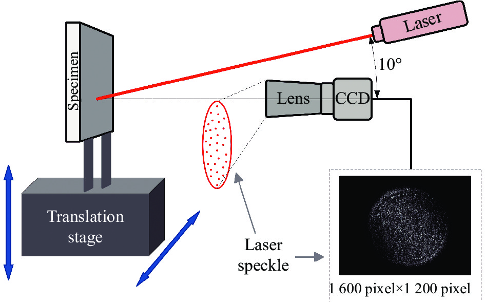
激光散斑图像采集装置示意图如图2所示,该装置主要包括半导体激光器(635 nm、1 mW)、CCD相机(190万 pixel)、远心镜头、激光器专用恒流电源、平移台。
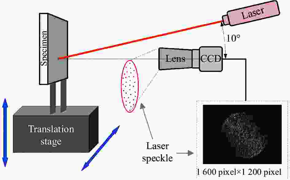
图 2 激光散斑图像采集装置示意图
Figure 2. Schematic diagram of laser speckle image acquisition device
采集的激光散斑图像与激光的入射角度、散射表面相对于激光的位置、激光功率及激光光斑的大小都有关系。该实验半导体激光器功率固定为1 mW,入射角度固定为与粗糙度试件表面法向呈10°,这确保了散射表面相对于激光始终处于相同的角度和位置,激光光斑大小始终不变。CCD相机和远心镜头用于记录散斑图案,带有镜头的CCD相机位于粗糙度试件表面的法线方向,与试件表面的距离固定为110 mm,这确保了观测平面在整个实验过程中都是一致的,并且相机接收到的镜面反射光较小,有效避免了相机信号饱和。实验中通过控制二维平移台移动试件,采集试件表面的散斑图像,每次曝光时都确保二维平移台和试件是静止的,整个过程中无需移动激光器,也不会影响其相对于散射表面的方向和位置。
-
实验选用平磨、卧铣、立铣、研磨四种不同加工工艺的粗糙度标准试件,共计15个标准试件。对每一个标准试件采集46张散斑图像,共计采集690张散斑图像。将采集的散斑图像划分为训练集和测试集,具体的样本划分如表2所示。
表 2 数据集样本划分
Table 2. Dataset sample division
Data set PG HM VM GP Training set 160 160 160 120 Test set 24 24 24 18 -
激光照射粗糙度标准试件,相机采集到的图像中除了激光散斑图案外还有背景区域。为消除边缘效应,保留像素大小为500 pixel×500 pixel的区域作为激光散斑图案的有效部分。然后用高斯滤波过滤图像中的噪声,预处理后的部分激光散斑图像见图3。

图 3 预处理后的激光散斑图像(平磨试件)。(a) Ra=0.1 μm; (b) Ra=0.2 μm; (c) Ra=0.4 μm; (d) Ra=0.8 μm
Figure 3. Preprocessed laser speckle images (Plane grinding specimens). (a) Ra=0.1 μm; (b) Ra=0.2 μm; (c) Ra=0.4 μm; (d) Ra=0.8 μm
-
从预处理后的激光散斑图像中提取了27个原始特征参数。灰度共生矩阵法提取了0°、45°、90°、135°方向的能量、熵、惯性矩、相关性和逆差矩特征,但是这样得到的特征参数过于繁多,取4个方向的平均值作为灰度共生矩阵的特征参数值。然后,引入斯皮尔曼相关系数,设置门限值Q为0.8,如果特征参数与各加工类型的表面粗糙度参数Ra之间的斯皮尔曼相关系数绝对值均高于门限值,则保留该特征参数,否则剔除该特征参数。各特征参数与表面粗糙度参数Ra之间的斯皮尔曼相关系数绝对值如表3所示。
表 3 特征参数与表面粗糙度参数之间的斯皮尔曼相关系数绝对值
Table 3. The absolute value of Spearman's correlation coefficient between feature parameters and surface roughness parameter
Process E S I L H Mmean PG 0.968 0.968 0.968 0.790 0.968 0.968 HM 0.968 0.968 0.968 0.968 0.968 0.799 VM 0.968 0.968 0.968 0.809 0.968 0.252 GP 0.943 0.943 0.935 0.928 0.943 0.943 Process Acon Bent D κ σ υ PG 0.968 0.968 0.968 0.968 0.968 0.968 HM 0.770 0.968 0.657 0.968 0.968 0.968 VM 0.284 0.945 0.177 0.959 0.968 0.968 GP 0.943 0.943 0.807 0.943 0.935 0.943 从表3可以看出,L与平磨试件表面粗糙度参数的相关性低于门限值,Mmean、Acon、D与卧铣和立铣试件表面粗糙度参数的相关性低于门限值,因此剔除L、Mmean、Acon、D,4个特征参数。经过预筛选后,筛选出的8个特征参数均与各加工类型表面粗糙度参数Ra有强相关性,记为:TV ={E, S, I, H, Bent, κ, σ, υ}。
-
经过特征参数的预筛选后,分别对平磨、卧铣、立铣、研磨试件表面建立基于多特征参数TV ={E, S, I, H, Bent, κ, σ, υ}的SVR模型,以实现四种加工类型表面粗糙度的测量,建模过程中不敏感函数参数取值为ε = 0.01。SVR模型的超参数和输入特征均会影响模型的性能。
优先考虑超参数对模型性能的影响,SVR模型的正则化系数C和核函数参数g会对模型的性能产生重要影响。文中利用5折交叉验证和网格搜索法对模型的超参数C和g进行寻优,各SVR模型最优的C和g如表4所示。将各加工类型的测试集数据分别输入到相应的SVR模型中,模型对测试集样本表面粗糙度预测的RMSE和MAPE如表5所示。
表 4 8输入特征SVR模型的最优C和g
Table 4. Optimal C and g of the SVR model with 8 input feature parameters
Hyper parameter PG HM VM GP C 3.7321 48.5029 0.8706 4.5948 g 0.0544 0.0718 8.0000 1.7411 表 5 8输入特征SVR模型的预测误差
Table 5. Prediction error of the SVR model with 8 input feature parameters
Process RMSE of the test set/μm MAPE of the test set PG 0.0151 4.77% HM 0.0375 3.72% VM 0.1979 8.16% GP 0.0022 3.88% 从表5可知,表面粗糙度测量模型的输入特征为TV ={E, S, I, H, Bent, κ, σ, υ}时,在最优超参数下,表面粗糙度测量模型对平磨、卧铣、立铣、研磨测试集样本预测的平均绝对百分比误差分别为4.77%、3.72%、8.16%和3.88%。
此外,输入特征也会影响表面粗糙度测量模型的性能,采用文中改进的序列后向选择算法来解决输入特征的冗余问题。选择5折交叉验证的最小均方误差函数为各SVR模型的性能评价函数,各SVR模型性能评价函数的阈值上限设置为输入特征全集时性能评价函数值的1.1倍。该算法依次从各SVR模型中剔除了冗余特征H、κ和σ。此时,表面粗糙度测量模型的输入特征数为5,记为TW ={E, S, I, Bent, υ},各SVR模型最优的$C$和$g$如表6所示。
表 6 5输入特征SVR模型的最优C和g
Table 6. Optimal C and g of the SVR model with 5 input feature parameters
Hyper parameter PG HM VM GP C 2.8284 48.5029 1.6245 4.2871 g 0.0769 0.1015 1.6245 2.2974 将各加工类型的测试集数据分别输入到相应的SVR模型中,模型对测试集样本表面粗糙度预测的RMSE和MAPE如表7所示。
表 7 5输入特征SVR模型的预测误差
Table 7. Prediction error of the SVR model with 5 input feature parameters
Process RMSE of the test set/μm MAPE of the test set PG 0.0148 3.55% HM 0.0371 3.10% VM 0.0532 3.17% GP 0.0016 2.27% 文中改进的序列后向选择算法把各SVR模型的输入特征数从8降低到了5,剔除冗余特征的同时,各SVR模型保留了相同的特征子集。此外,从表5和表7可知,该方法还将平磨、卧铣、立铣、研磨SVR模型的MAPE分别降低了1.22%、0.62%、4.99%、1.61%,模型的RMSE也更低,具有更高的准确性和稳定性。
测试集样本表面粗糙度标准值和预测值如图4所示,预测结果的相对误差如图5所示。从图5可知,平磨0.1~0.8 μm粗糙度等级的样本,表面粗糙度预测的最大相对误差为9.85%;卧铣和立铣0.4~3.2 μm粗糙度等级的样本,表面粗糙度预测的最大相对误差为7.10%和7.95%;研磨0.025~0.1 μm粗糙度等级的样本,表面粗糙度预测的最大相对误差为9.21%,对各加工类型的表面粗糙度的最大相对误差均小于10%。
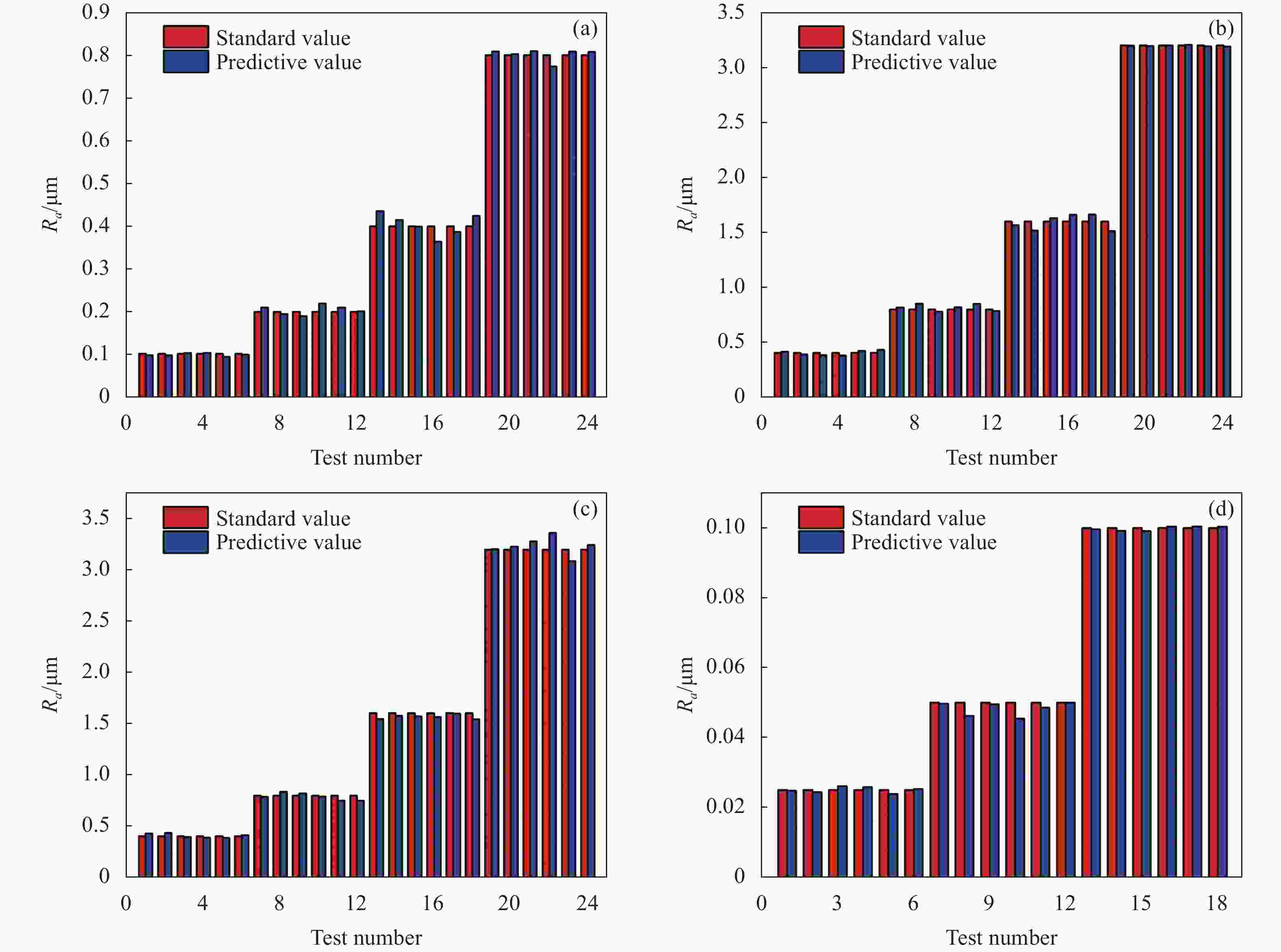
图 4 测试集表面粗糙度标准值和预测值。(a)平磨;(b)卧铣;(c)立铣;(d)研磨
Figure 4. Standard and predicted values of surface roughness for the test set. (a) Plane grinding; (b) Horizontal milling; (c) Vertical milling; (d) Grinding polishing

图 5 表面粗糙度预测的相对误差图。(a)平磨;(b)卧铣;(c)立铣;(d)研磨
Figure 5. Relative error graph of surface roughness prediction. (a) Plane grinding; (b) Horizontal milling; (c) Vertical milling; (d) Grinding polishing
前述已用筛选出的特征参数TW ={E, S, I, Bent, υ}建立了测量各加工类型表面粗糙度的模型,由于各模型的支持向量回归函数不同,因此需要确定加工类型后,才能代入相应的SVR模型进行表面粗糙度测量。基于特征参数TW ={E, S, I, Bent, υ}建立了SVM分类器和K最近邻(K-Nearest Neighbor, KNN)分类器。分类器对测试集样本加工类型的预测结果如表8和表9所示,表格的行表示实际类别,列表示预测类别。
表 8 SVM分类器预测结果的混淆矩阵
Table 8. The confusion matrix of the prediction results by the SVM classifier
Process PG HM VM GP PG 24 0 0 0 HM 0 24 0 0 VM 0 0 24 0 GP 0 0 0 18 表 9 KNN分类器预测结果的混淆矩阵
Table 9. The confusion matrix of the prediction results by the KNN classifier
Process PG HM VM GP PG 24 0 0 0 HM 0 23 0 1 VM 0 0 24 0 GP 0 1 0 17 从表8和表9可知,基于特征参数TW ={E, S, I, Bent, υ}建立的SVM分类器和KNN分类器对测试集样本加工类型的识别率分别为100%和97.78%。由于需要根据识别的加工类型代入相应的SVR模型实现表面粗糙度的测量,因此对加工类型识别率要求较高,通过对比后,文中选择建立的SVM分类器作为加工类型识别的模型。
-
文中提出了一种解决表面粗糙度建模过程中特征相关和特征冗余问题的方法。通过引入斯皮尔曼相关系数,制定简约规则,可以筛选出与各加工类型表面粗糙度参数均强相关的特征参数,改进的序列后向选择算法,解决了模型的特征冗余问题。实验结果表明,文中提出的方法不仅有效剔除了不相关特征和冗余特征,还可以筛选出一组特征TW ={E, S, I, Bent, υ},建立适用于测量各加工类型表面粗糙度的模型。建立的模型对四种加工类型的识别率为100%,对平磨、卧铣、立铣和研磨表面粗糙度预测的MAPE分别为3.55%、3.10%、3.17%、2.27%,对表面粗糙度有较高的测量精度,与剔除冗余特征前相比,平磨、卧铣、立铣和研磨SVR模型的MAPE分别降低了1.22%、0.62%、4.99%、1.61%,模型的准确性和稳定性更优。
Research on surface roughness modeling based on multiple feature parameters of laser speckle image
-
摘要: 散斑法是表面粗糙度测量领域的研究热点之一,该方法可以通过建立散斑图像特征参数与表面粗糙度评定参数之间的关系,实现对工件表面粗糙度的高效和无损测量。然而,该方法在特征参数选取阶段缺乏统一的标准,工件的机加工方法也会对特征参数和表面粗糙度评定参数之间的关系产生影响。这可能导致选取的特征参数仅适用于某种加工工艺下的表面粗糙度测量,并且特征参数之间还可能存在冗余问题。针对以上问题,文中从采集的激光散斑图像中提取了多个特征参数,引入斯皮尔曼相关系数,制定简约规则对提取的特征参数进行预筛选,提出了改进的序列后向选择算法以剔除冗余特征。实验结果表明:文中提出的方法筛选出了一组与不同加工工艺的表面粗糙度均强相关的特征,并解决了特征冗余问题,利用这组特征建立的表面粗糙度测量模型能100%识别试件的加工类型,并实现对其表面粗糙度较高精度的测量,改进的序列后向选择算法将平磨、卧铣、立铣和研磨试件表面粗糙度测量模型的平均绝对百分比误差分别降低了1.22%、0.62%、4.99%和1.61%,解决特征冗余问题的同时建立的模型性能更优。Abstract:
Objective Speckle method stands out as one research hotspots in the realm of surface roughness measurement, boasting advantages such as low loss, high-temperature resistance, and high reliability. As the scenarios for surface roughness measurement grow in complexity and precision requirements continue to escalate, a novel surface roughness modeling method based on multiple feature parameters of laser speckle images has been proposed. This method is grounded in multiple feature parameters extracted from laser speckle images. However, the modeling process using this approach confronts challenges related to feature correlation and redundancy. The presence of irrelevant or redundant features in the modeling process can result in prelonged feature extraction times, heightened computational costs, and increased model complexity. Furthermore, these features can detrimentally affect the accuracy and stability of the model. To address these issues, a method is proposed to alleviate feature correlation and redundancy during surface roughness modeling. Simultaneously, the selected features are designed to facilitate the measurement of surface roughness across various processing types. Methods Introducing Spearman's correlation coefficient, we aim to establish succinct rules for the effective screening of laser speckle image feature parameters that exhibit strong correlations with the surface roughness evaluation parameter Ra for each processing type (Tab.1). To address redundancy among feature parameters, an enhanced sequential backward selection algorithm is employed. Subsequently, laser speckle images from various peocessing types, including plane grinding, horizontal milling, vertical milling, and grinding polishing standard specimens, were acquired through experiments (Fig.2, Fig.3). Utilizing these collected laser speckle images, we constructed a surface roughness measurement model based on support vector machines. The method's efficacy was then validated through comprehensive verification processes. Results and Discussions From the gathered later speckle images, a total of 27 feature parameters were initially extracted. By introducing Spearman's correlation coefficient and formulating simple rules, we identified 8 feature parameters {E, S, I, H, Bent, κ, σ, υ} strongly correlated with the surface roughness evaluation parameter Ra for each processing type. Then, redundant feature parameters H, κ and σ were effectively eliminated using an improved sequence backward selection algorithm. This process not only addressed the issues of feature correlation and redundancy but also led to the establishment of a surface roughness measurement model incorporating the selected feature parameters{E, S, I, Bent, υ}. The resulting model demonstrated a remarkable 100% recognition rate for processing type and exhibited high-precision measurement of surface roughness (Tab.7, Tab.8). In addition, the enhanced sequential backward selection algorithm contributed to a reduction in the MAPE for the surface roughness measurement model across different specimens: plane grinding, horizontal milling, vertical milling, and grinding polishing. The reductions were 1.22%, 0.62%, 4.99% and 1.61%, respectively. Conclusions The proposed method effectively addresses the issues of feature correlation and redundancy in the process of surface roughness modeling, leveraging multiple feature parameters extracted from laser speckle images. By eliminating irrelevant and redundant features, the method prevents unnecessary consumption of feature extraction time and reduces model calculation costs. The resulting model exhibits enhanced stability and accuracy. Experimental results demonstrate the effectiveness of the model established using the selected feature parameters. It achieves a 100% recognition rate for processing types such as plane grinding, horizontal milling, vertical milling, and grinding polishing specimens. Moreover, the MAPE for surface roughness prediction is reduced to 3.55%, 3.10%, 3.17%, and 2.27%, respectively. These reductions represent improvements of 1.22%, 0.62%, 4.99%, and 1.61% compared to the model's perfomance before removing redundant features. -
图 1 表面粗糙度测量模型的建模过程
Figure 1. The modeling process of surface roughness measurement model
图 2 激光散斑图像采集装置示意图
Figure 2. Schematic diagram of laser speckle image acquisition device
图 3 预处理后的激光散斑图像(平磨试件)。(a) Ra=0.1 μm; (b) Ra=0.2 μm; (c) Ra=0.4 μm; (d) Ra=0.8 μm
Figure 3. Preprocessed laser speckle images (Plane grinding specimens). (a) Ra=0.1 μm; (b) Ra=0.2 μm; (c) Ra=0.4 μm; (d) Ra=0.8 μm
图 4 测试集表面粗糙度标准值和预测值。(a)平磨;(b)卧铣;(c)立铣;(d)研磨
Figure 4. Standard and predicted values of surface roughness for the test set. (a) Plane grinding; (b) Horizontal milling; (c) Vertical milling; (d) Grinding polishing
图 5 表面粗糙度预测的相对误差图。(a)平磨;(b)卧铣;(c)立铣;(d)研磨
Figure 5. Relative error graph of surface roughness prediction. (a) Plane grinding; (b) Horizontal milling; (c) Vertical milling; (d) Grinding polishing
表 1 材料和表面粗糙度参数
Table 1. Material and surface roughness parameters
Set Process Material Standard value of surface roughness Ra/μm PG Plane grinding 45#steel 0.1 0.2 0.4 0.8 HM Horizontal milling 45#steel 0.4 0.8 1.6 3.2 VM Vertical milling 45#steel 0.4 0.8 1.6 3.2 GP Grinding polishing GCr15 0.025 0.05 0.1 -  下载: 导出CSV
表 2 数据集样本划分
Table 2. Dataset sample division
Data set PG HM VM GP Training set 160 160 160 120 Test set 24 24 24 18
下载: 导出CSV
表 3 特征参数与表面粗糙度参数之间的斯皮尔曼相关系数绝对值
Table 3. The absolute value of Spearman's correlation coefficient between feature parameters and surface roughness parameter
Process E S I L H Mmean PG 0.968 0.968 0.968 0.790 0.968 0.968 HM 0.968 0.968 0.968 0.968 0.968 0.799 VM 0.968 0.968 0.968 0.809 0.968 0.252 GP 0.943 0.943 0.935 0.928 0.943 0.943 Process Acon Bent D κ σ υ PG 0.968 0.968 0.968 0.968 0.968 0.968 HM 0.770 0.968 0.657 0.968 0.968 0.968 VM 0.284 0.945 0.177 0.959 0.968 0.968 GP 0.943 0.943 0.807 0.943 0.935 0.943
下载: 导出CSV
表 4 8输入特征SVR模型的最优C和g
Table 4. Optimal C and g of the SVR model with 8 input feature parameters
Hyper parameter PG HM VM GP C 3.7321 48.5029 0.8706 4.5948 g 0.0544 0.0718 8.0000 1.7411
下载: 导出CSV
表 5 8输入特征SVR模型的预测误差
Table 5. Prediction error of the SVR model with 8 input feature parameters
Process RMSE of the test set/μm MAPE of the test set PG 0.0151 4.77% HM 0.0375 3.72% VM 0.1979 8.16% GP 0.0022 3.88%
下载: 导出CSV
表 6 5输入特征SVR模型的最优C和g
Table 6. Optimal C and g of the SVR model with 5 input feature parameters
Hyper parameter PG HM VM GP C 2.8284 48.5029 1.6245 4.2871 g 0.0769 0.1015 1.6245 2.2974
下载: 导出CSV
表 7 5输入特征SVR模型的预测误差
Table 7. Prediction error of the SVR model with 5 input feature parameters
Process RMSE of the test set/μm MAPE of the test set PG 0.0148 3.55% HM 0.0371 3.10% VM 0.0532 3.17% GP 0.0016 2.27%
下载: 导出CSV
表 8 SVM分类器预测结果的混淆矩阵
Table 8. The confusion matrix of the prediction results by the SVM classifier
Process PG HM VM GP PG 24 0 0 0 HM 0 24 0 0 VM 0 0 24 0 GP 0 0 0 18
下载: 导出CSV
表 9 KNN分类器预测结果的混淆矩阵
Table 9. The confusion matrix of the prediction results by the KNN classifier
Process PG HM VM GP PG 24 0 0 0 HM 0 23 0 1 VM 0 0 24 0 GP 0 1 0 17
下载: 导出CSV
-
[1] 陈苏婷, 张勇, 胡海锋. 基于激光散斑分形维数的表面粗糙度测量方法[J]. 中国激光, 2015, 42(4): 0408002. doi: 10.3788/cjl201542.0408002 Chen Suting, Zhang Yong, Hu Haifeng. Surface roughness measurement based on fractal dimension of laser speckle [J]. Chinese Journal of Lasers, 2015, 42(4): 0408002. (in Chinese) doi: 10.3788/cjl201542.0408002 [2] 刘颖, 朗 治 国, 唐 文 彦. 表面粗糙度光切显微镜测量系统的研制[J]. 红外与激光工程, 2012, 41(3): 775-779. Liu Ying, Lang Zhiguo, Tang Wenyan. Development of measurement system about light-section microscope for surface roughness [J]. Infrared and Laser Engineering, 2012, 41(3): 775-779. (in Chinese) [3] Gontard L C, López-castro J D, González-rovira L, et al. Assessment of engineered surfaces roughness by high-resolution 3 D SEM photogrammetry [J]. Ultramicroscopy, 2017, 177: 106-114. doi: 10.1016/j.ultramic.2017.03.007 [4] Misumi I, Sugawara K, Kizu R, et al. Extension of the range of profile surface roughness measurements using metrological atomic force microscope [J]. Precision Engineering, 2019, 56: 321-329. doi: 10.1016/j.precisioneng.2019.01.002 [5] Niemczewska-wójcik M, Madej M, Kowalczyk J, et al. A comparative study of the surface topography in dry and wet turning using the confocal and interferometric modes [J]. Measurement, 2022, 204: 112144. doi: 10.1016/j.measurement.2022.112144 [6] Chen H R, Chen L C. Full-field chromatic confocal microscopy for surface profilometry with sub-micrometer accuracy [J]. Optics and Lasers in Engineering, 2023, 161: 107384. doi: 10.1016/j.optlaseng.2022.107384 [7] Song I U, Yang H S, Kim G, et al. Surface form error measurement for rough surfaces using an infrared lateral shearing interferometry [J]. Optics and Lasers in Engineering, 2022, 152: 106947. doi: 10.1016/j.optlaseng.2022.106947 [8] Zou Y, Li Y, Kaestner M, et al. Low-coherence interferometry based roughness measurement on turbine blade surfaces using wavelet analysis [J]. Optics and Lasers in Engineering, 2016, 82: 113-121. doi: 10.1016/j.optlaseng.2016.02.011 [9] Manallah A, Bouafia M. Application of the technique of total integrated scattering of light for micro-roughness evaluation of polished surfaces [J]. Physics Procedia, 2011, 21: 174-179. doi: 10.1016/j.phpro.2011.10.026 [10] Han W, Lim J, Lee S J, et al. Bidirectional reflectance distribution function (BRDF)-based coarseness prediction of textured metal surface [J]. IEEE Access, 2022, 10: 32461-32469. doi: 10.1109/ACCESS.2022.3161518 [11] Patil S H, Kulkarni R. Objective speckle pattern-based surface roughness measurement using matrix factorization [J]. Applied Optics, 2022, 61(32): 9674-9684. doi: 10.1364/AO.473076 [12] 蒋磊, 刘恒彪, 李同保. 超辐射发光二极管的散斑自相关法表面粗糙度测量研究[J]. 红外与激光工程, 2019, 48(7): 717003-0717003(7). doi: 10.3788/IRLA201948.0717003 Jiang Lei, Liu Hengbiao, Li Tongbao. Research on surface roughness measurement of speckle autocorrelation method based on SLD [J]. Infrared and Laser Engineering, 2019, 48(7): 0717003. (in Chinese) doi: 10.3788/IRLA201948.0717003 [13] Persson U. Roughness measurement of machined surfaces by means of the speckle technique in the visible and infrared regions [J]. Optical Engineering, 1993, 32(12): 3327-3332. doi: 10.1117/12.151303 [14] Patel D R, Vakharia V, Kiran M B. Texture classification of machined surfaces using image processing and machine learning techniques [J]. FME Transactions, 2019, 47(4): 865-872. doi: 10.5937/fmet1904865P [15] Patel D R, Kiran M B. Non-contact surface roughness measurement using laser speckle technique [J]. IOP Conference Series: Materials Science and Engineering, 2020, 895(1): 012007. [16] Chen Suting, Hu Haifeng, Zhang Chuang. Surface roughness modeling based on laser speckle imaging [J]. Acta Physica Sinica, 2015, 64(23): 234203. (in Chinese) doi: 10.7498/aps.64.234203 [17] Goh C S, Ratnam M M. Assessment of areal (Three-Dimensional) roughness parameters of milled surface using charge-coupled device flatbed scanner and image processing [J]. Experimental Techniques, 2016, 40(3): 1099-1107. doi: 10.1007/s40799-016-0111-z [18] Haridas A, Crivoi A, Prabhathan P, et al. Fractal speckle image analysis for surface characterization of aerospace structures[C]//International Conference on Optical & Photonics Engineering, 2017, 10449: 329-336. [19] Shao M, Xu D, Peng G, et al. A multiparameter surface roughness evaluation model of cold-rolled strips using laser speckle images [J]. Measurement, 2022, 203: 111991. doi: 10.1016/j.measurement.2022.111991 [20] Goodman J W. Speckle Phenomena in Optics: Theory and Applications[M]. US: Roberts and Company Publishers, 2014: 9-11. -

 点击查看大图

计量
- 文章访问数: 107
- HTML全文浏览量: 21
- PDF下载量: 29
- 被引次数: 0

