光学偏折术(Phase measurement deflectometry, PM-D)因其结构简单、检测精度高、范围大等优点被用于自由曲面透射式波前检测，高精度的相位获取是测量检测过程的关键步骤之一。相位解包裹是光学领域中一项重要而具有挑战性的任务，它在光学干涉测量、磁共振成像、条纹投影轮廓测量等领域中扮演着关键的角色^[1−4]。其挑战在于从观测到的[−$ \pi $,$ \pi $)范围内的包裹相位信号中恢复成连续变化的真实相位信号。

理想情况下，相位展开可以根据相邻像素之间的相位差，通过在每个像素处加减2$ \pi $来完成。然而，在实践中由于包裹相位存在噪声、相位不连续等问题，造成了包裹相位中极点的存在^[5]。极点会导致解包裹路径中累积计算误差，从而导致相位展开失败。为了得到真实的相位分布，就需要采用各种方法对包裹相位进行解包裹处理。

现有的相位解包裹方法包括路径跟踪算法和路径无关算法^[6]。路径跟踪算法，如质量导向图相位展开（Quality guided phase unwrap, QGPU）^[6]算法和枝切算法^[7]（Goldstein’s branch cut algorithm），通过按特定路径展开相位，根据质量判断出最佳路径。尽管路径跟踪算法的计算效率相对较高，但是它对噪声缺少鲁棒性，限制了其应用场景；路径无关算法，如傅里叶变换法^[5]和最小二乘法^[8]，虽然对于噪声的鲁棒性较好，但是该算法计算复杂度高，迭代收敛慢、运算效率低，对于大规模相位数据和高分辨率图像，需要较长的计算时间和较大的计算资源。实际上，传统空间相位解包裹的目的都是尽可能地避免无效点的负面影响，主要适用于非严重噪声和一些离散的不连续点。但是在一些极端情况下，例如存在严重噪声或局部孤立的不连续区域，传统方法将变得无效。

近年来，深度学习算法得到了普及，已经被广泛地应用于目标检测和图像分类任务中^[9]。遵循这一发展趋势，研究试图应用深度学习来解决相位解包裹问题。

其中，Jin等人首先提出使用深度学习来解决光学成像中的相位展开问题^[10]。这种使用深度神经网络学习从输入空间到输出空间的映射关系的想法，使得解决空间相位解包裹问题成为可能； Spoorthi G E^[11]和Zhang T^[12]等人将相位展开问题重新表述为语义分割任务，其中训练全卷积网络(Fully convolutional network, FCN)来预测每个展开相位的包裹计数。然而，全卷积网络在下采样时存在损失细节信息问题，且网络收敛速度较慢，往往需要大量的数据集，从而限制了其在实际中的应用；Wang等人提出基于U-Net的语义分割模型（Deep learning phase unwrapping, DLPU）^[13], 通过引入跳跃连接和增加特征通道的方式，通过在模拟数据集上的测试，在相位解包裹任务中相比全卷积网络取得了更好的性能；2022年，Zhou^[14]等设计一种基于对抗神经网络的解包裹技术，以提高传统方法的鲁棒性和有效性；同年，Xu^[15]等人提出了MNet网络，通过丰富的跳跃连接结构，促进浅层信息和深层特征的融合，同时使用结构损失函数。然而，由于卷积神经网络(CNN)中的卷积操作和池化操作仅关注局部窗口内的像素^[16]，忽略了图像不同区域之间的全局空间关系和整个图像的全局结构。由于大多数真实世界的相位图像都包含一定的空间结构，因此在学习从包裹相位到绝对相位的映射时，对这种全局空间关系进行建模是至关重要的。

循环神经网络(Recurrent neural network, RNN) ^[17]是一种可以对时间序列内的上下文关系进行建模的神经网络。Ryu等人首先尝试使用卷积和传统循环神经网络的组合在MRI图像中执行相位展开^[18]。然而，这项研究并没有做定量分析；Perera等人^[19] 虽然考虑到噪声情况的解包裹相位，但是缺乏对极端条件(像不连续与混叠)下的研究。

针对上述问题，文中提出了一种基于改进U-Net网络的相位解包裹算法。该算法以U-Net网络作为基础网络，添加可以对时间序列建模的CBiLSTM模块；同时引入注意力机制，增加模型的泛化能力和可解释性；通过对损失函数的对比与改进，找出最适合应用于本研究的损失函数。最后，将提出的网络模型同时经过模拟数据集和真实数据集验证，证明其在噪声、不连续、混叠三种情况下的优秀性能。

注意力机制的引入，可以更好地捕捉图像的全局空间关系；CBiLSTM通过记忆单元结构，能够有效地捕捉和存储长期依赖关系。相比于传统神经网络，记忆单元可以选择性地记住和忘记输入信号的部分信息，从而能够更好地处理长序列数据的建模任务。

在模型训练过程中，根据空间相位解包裹这一特定问题，定义了一个复合损失函数来训练网络。

将文中提出的网络同U-Net^[20]、Res-UNet^[21]等经典网络模型还有Wang^[13]、Perera等人^[19]提出的方法做比较实验，验证文中所提出的网络对严重噪声和不连续的条件具有很强的鲁棒性，并且在执行空间相位解包裹任务时具有很高的计算效率。

文中使用的数据集分为模拟数据集和真实数据集两部分，模拟数据集用于训练与验证网络的性能，真实数据集用于验证网络的泛化能力。

文中使用的真实绝对相位数据集来自实际样品，通过对其进行强度传输方程^[10]的再处理得到包裹相位；使用的模拟数据集由包含随机形状的合成相位图像及其相应的包裹相位图像组成。这些随机形状是通过增加和减少几个具有不同形状和位置的高斯函数而产生的。使用高斯函数保证生成的模拟数据集的连续性，同时通过高斯参数的变化和随机函数的叠加引入随机性。

绝对相位$ \varphi \left(x,y\right) $和包裹相位$ \psi \left(x,y\right) $计算如下：

式中：j为虚数单位。

按照这种方法，创建了三个数据集，每个数据集由2000幅相位图像(256×256)组成，其值范围为随机选择从−44~44，分别作为包裹相位与绝对相位，如图1所示。第一个数据集在包裹相位被包裹之前随机赋予[0,5,10,20,80]的高斯噪声，以分别模拟真实数据中无噪声、轻度噪声、中度噪声、严重噪声的情况。第二个数据集把包裹相位被包裹之前在无噪声条件下赋予一个大小、位置随机且相位值也随机的矩形区域，来模拟真实数据中包裹相位不连续的情况。

图  1  （a）绝对相位(真实数据集)；（b） 包裹相位(真实数据集)；（c）绝对相位(模拟数据集1,2)；（d）包裹相位(模拟数据集1)；（e）包裹相位(模拟数据集2)；（f）包裹相位(模拟数据集3)

Figure 1.  （a） Absolute phase (real data set); （b） Wrapped phase (real data set); （c） Absolute phase (simulated data set 1, 2); （d） Wrapped phase (simulated data set 1); （e） Wrapped phase (simulated data set 2); （f） Wrapped phase (simulated data set 3)

第三个数据集将前两种情况混叠在一起，同时将不连续和噪声加入到包裹相位中，来模拟真实数据中更复杂的混叠情况。

香浓熵(Shannon entropy) ^[22]是信息论中用来衡量数据集不确定性的指标，它可以定量表征数据集中包含的信息量。影响训练后神经网络的泛化能力，香浓熵的计算公式如下：

式中：$ P\left({a}_{i}\right) $为某一事件发生的概率，其中对数一般取2为底，单位为bit。

通过计算数据集1和数据集2绝对相位的香浓熵，熵的平均值分别为4.65、5.50，如图2所示。这个结果初步表明，模拟数据集在信息丰富程度上接近真实数据集。

图  2  真实数据与模拟数据香浓熵的比较

Figure 2.  Comparison of Shannon entropy between real and simulated dataset

归一化均方根误差（Normalized root mean square error, NRMSE）是一种评价预测结果与真实结果之间差异的指标，常用于回归问题的模型评估。它将均方根误差（RMSE）归一化到预测值的范围内，使得不同数据集和问题之间的比较更为公平。NRMSE的公式如下：

式中：MSE 为均方误差；$ {y}_{\max} $ 和 $ {y}_{\min} $分别为预测值和真实值的最大最小值。

峰值信噪比（Peak signal-to-noise ratio, PSNR）是评估图像质量的一种指标，常用于图像压缩和图像增强等领域。PSNR 表示预测图像与原始图像之间的峰值信噪比，用来衡量图像失真的程度，数值越高表示图像质量越好。

PSNR的公式如下：

式中：S 为图像像素值的最大可能取值。

结构相似性指数（Structural similarity index, SSIM）是一种评估图像相似性的指标，常用于图像质量评估和图像比较。它同时考虑了亮度、对比度和结构的相似性，可以更好地反映人眼感知的图像质量差异。SSIM的公式如下：

式中：x 和 y 分别表示预测绝对相位和真实绝对相位；$ \mu $表示均值；$ \sigma $ 表示标准差；$ \sigma_{xy} $ 表示协方差；$ c_{1} $ 和 $ c_{2} $为常数，用来避免分母为零。

相位展开可以被看成是一个回归问题，根据输入的有噪声或者不连续的包裹相位来预测出绝对相位。为了准确地识别类别，文中引入了一种基于图像的语义分割的网络框架。网络的设计如图3所示。该网络包括编码器和解码器、CBiLSTM模块、软注意力机制模块，网络中的每个卷积块包含两个3×3的卷积层，两个批处理归一化层和两个ReLU激活。每个编码器卷积块后面都有一个2×2的平均池化层，步幅为2，而每个解码器卷积块前面都有一个3×3的转置卷积层，步幅为2。由于网络执行回归任务，因此解码器层的最后一个卷积块由一个线性激活的1×1卷积层接替。

图  3  网络模型图

Figure 3.  Network model diagram

其中，编码器的输出馈送到解码器之前通过所提出的CBiLSTM模块。编码器的输出特征映射能够表示输入图像的局部信息。然后，将这个编码器的输出输入到CBiLSTM模块中，网络可以学习编码器输出中包含的局部特征之间的空间依赖关系。随后，将CBiLSTM模块的输出送入到解码器网络中。解码器包含一系列转置卷积层和跳跃连接组成；其中，转置卷积层逐渐将低分辨率的特征图恢复为与输入图像大小相匹配的高分辨率特征图。跳跃连接用于传递来自编码器的低层特征，帮助解码器更好地还原细节。在解码器网络中添加软注意力机制模块，解码部分特征图与其对应的编码部分特征图作为注意力门（Attention gate）的输入，经过注意力门后将结果与上采样的编码部分作为解码器下一次的输入特征图。

和LSTM只考虑了过去的历史信息相比，BiLSTM结合了正向和反向两个方向的信息^[17]。这意味着Bi-LSTM可以同时利用当前位置之前和之后的上下文信息，从而更全面地理解输入序列，这对于预期相互依赖的系列是有利的。同时，BiLSTM有更好的特征提取能力，BiLSTM能够同时捕捉到局部和全局的依赖关系。正向传播捕获了局部的前向依赖关系，而反向传播捕获了局部的后向依赖关系。结合这两个方向的依赖关系可以提供更丰富的特征表示，有助于更好地学习和捕捉序列中的模式。一个BiLSTM由两个LSTM组成，$ {{X}}_{\to } $为输入，$ {{X}}_{\leftarrow } $为反向重排。$ {{h}}_{{f}{o}{r}\to } $和$ {{h}}_{{b}{a}{c}{k}\leftarrow } $分别是相应的用LSTM处理$ {{X}}_{\to } $和$ {{X}}_{\leftarrow } $得到的输出。设$ {{h}}_{{b}{a}{c}{k}\leftarrow } $为按原顺序重新排列的输出，BiLSTM的输出如下：

文中提出了BiLSTM 2D层作为一种二维空间信息的方法，模型图如图4所示。该模块有两个普通的BiLSTM，一个垂直的BiLSTM和一个水平的BiLSTM和两个卷积层。

对于输入X=∈$ {M}_{W\times H\times B} $,$ {\{{X}_{:,W},:\in {{{{M}}}}^{H\times C}\}}_{H=1}^{W} $被视为一组序列，所有序列{:,W,:}都输入到垂直的BiLSTM中，共享权重和隐藏维度D，则：

用上述相似的方式，$ {\{{X}_{H,:,:}:\in {{M}}^{H\times C}\}}_{w=1}^{H} $被视为一组序列，所有序列{H,:,:}都输入到水平的BiLSTM中，共享权重和隐藏维度D，则：

然后，将经过卷积之后的$ {\{{H}_{:,W,:}^{ver}\in {{M}}^{H\times 2 D}\}}_{H=1}^{W} $和$ {\{{H}_{H,:,:}^{hor}\in {{M}}^{H\times 2 D}\}}_{w=1}^{H} $分别合并到$ {{H}}^{ver}\in {{M}}^{W\times H\times 2 D} $和$ {{H}}^{hor}\in {{M}}^{W\times H\times 2 D} $。

图  4  CBiLSTM模块示意图

Figure 4.  Schematic diagram of CBiLSTM module

文中提出的注意门（Attention gate）被放入整体架构中，以突出通过跳跃连接的显著特征。注意门有两个输入信号：一个是由跳跃连接传输的特征映射；另一个输入是由前一神经层的输出得到的粗特征。从上一层神经网络提取的粗特征信息用来消除跳跃连接中的不相关响应产生的歧义。注意门的输出连接到下一个解码器。每个跳跃连接的门控信号聚合了来自多个成像尺度的信息，这增加了注意力权重的分辨率，有助于实现更好的性能。

文中所提出的注意门如图5所示，它实际上是一个简单的编码器-解码器模式的子网。注意门由五个3×3卷积层、五个批处理归一化层、五个ReLU激活层、两个最大池化层和一个转置卷积层组成。

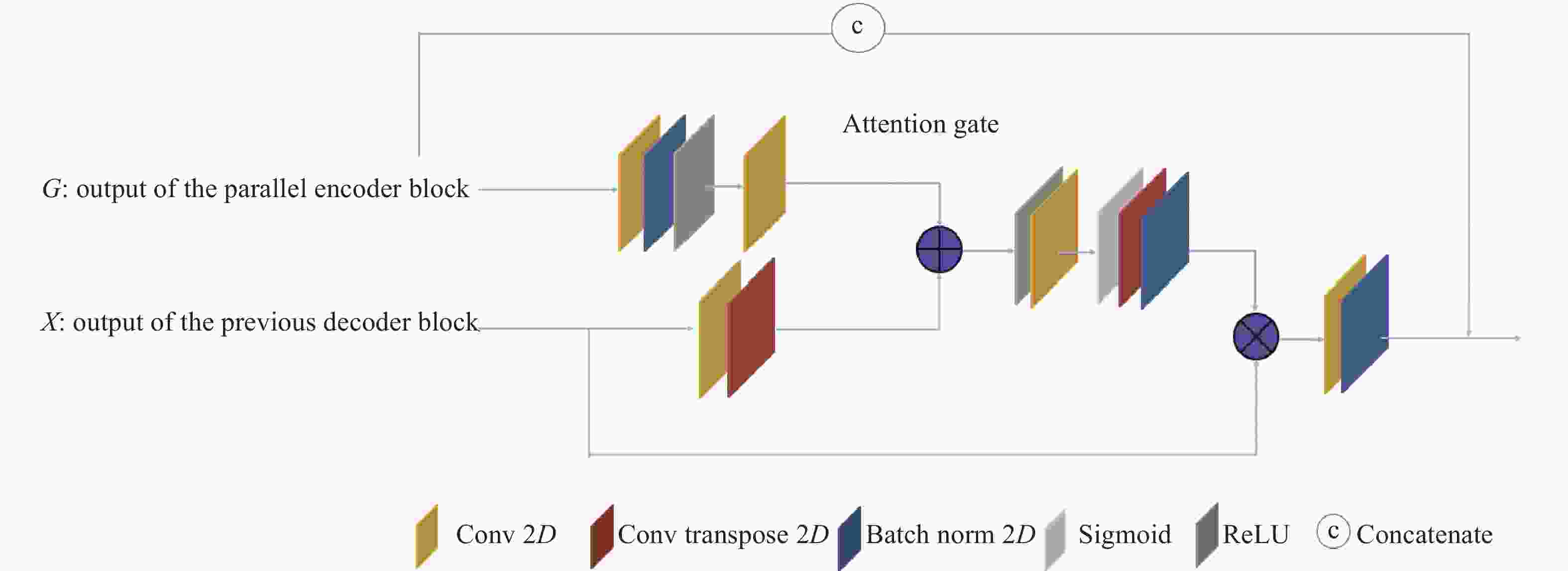
图  5  注意力门模块示意图

Figure 5.  Attention gate schematic

首先，g与$ {x}^{l} $进行并行操作，分别得到A、B，随后进行A+B操作得到C。然后C进行ReLU操作得到D，D进行sigmoid操作得到F，该层在范围[0,1]之间缩放向量，产生Attention系数(权重)，其中系数接近1表示更相关的特征。使用三线性插值将Attention系数（F）向上采样到x向量的原始维度。Attention系数按元素顺序与原始x向量相乘，根据相关性缩放向量F通过三线性插值重采样得到注意力系数α。最后，注意力系数α乘以$ {{x}}^{l} $得到$ {\widehat{x}}^{l} $。$ {\widehat{x}}^{l} $再经过卷积和归一化操作得到$ {\widehat{X}}^{l} $作为下一次的输入。

由于文中将相位展开问题表述为回归任务，因此损失函数的选择是MSE损失。然而，当将MSE损失应用于文中所提出的网络时，其收敛性不足，导致相位展开性能较差。包裹相位与绝对相位之间存在如下关系：

式中：r为矢量坐标；k为包裹计数，整数。通过公式（10）可以得到绝对相位$ \varphi +2\pi n $，其中$ \forall n\in Z $会产生相同的包裹相位$ \psi $。

由于$ \psi $的相位展开问题没有唯一解。因此，MSE损失迫使网络学习唯一解，它不适用于相位展开问题。所以，需要一个损失函数，它允许在收敛时的其他解，同时增加预测绝对相位$ \stackrel{~}{\varphi } $和真实绝对相位$ \varphi $之间的相似性。为了解决这些问题，采用下面定义的复合损失函数$ {L}_{new} $：

其中

式中：$ \alpha $、$ \beta $为这两种损失分配的权值，在训练时经验地分别设置为1和0.1。误差损失方差$ {L}_{mean} $允许在收敛时的替代解，而误差损失总变化$ {L}_{error} $通过强制网络匹配它们的梯度来增加$ \stackrel{~}{\varphi } $和$ \varphi $之间的相似性。

文中提出的网络在Keras中实现，并分别在上文提到的模拟数据集上进行了训练和测试。模型都使用学习率为0.001的ADAM优化器进行训练，以下模型训练的迭代次数均在500次以下，训练时长在3 h之内。

Res-UNet^[21]、Perera^[19]等人的网络、U-Net^[20]和Wang ^[13] 等人的网络也在这个数据集上实现和测试。以上实验均在混叠噪声、不连续、混叠情况下进行测试，以上所有训练和测试都是在R9000 p3060 GPU上进行的。

为了评估和比较这些方法，计算了未包裹相位图像的归一化均方根误差，通过各自真实相位图像的范围归一化，并记录了每种训练方法达到收敛状态所需要的训练轮次数。图6~8记录了每种网络模型分别在模拟数据集和真实数据集中的实验效果和网络性能。图6~9从左到右依次代表了原始包裹相位图、原始绝对相位图以及Res-UNet^[21]、文中提出的网络模型、U-Net^[20]、Wang ^[13] 等人提出的网络、Perera^[19]等人提出的网络模型的解包裹相位效果图。通过模拟数据集分别对网络模型在噪声、不连续、混叠情况下的相位解包裹能力的验证和真实数据集对网络模型泛化的验证。

图  6  各个网络模型在不同噪声情况下的性能

Figure 6.  The performance of each network model under different noise conditions

图  7  各个网络模型在不连续情况下的性能

Figure 7.  The performance of each network model in the case of discontinuity

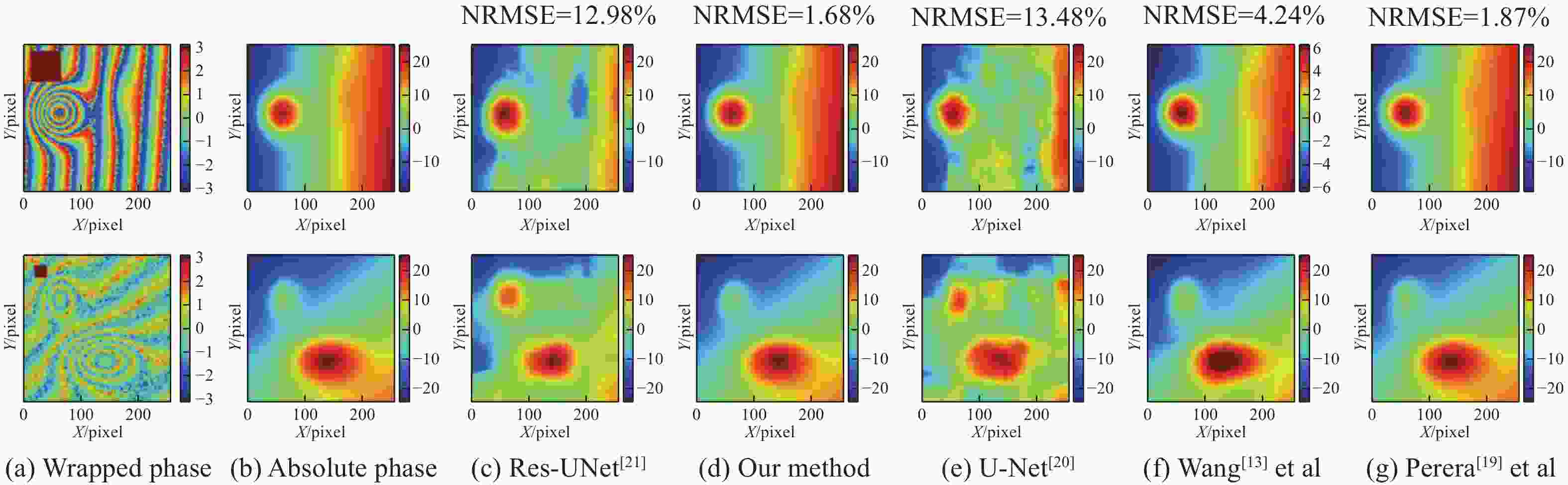
图  8  各个网络模型在混叠情况下的性能

Figure 8.  Performance of individual network models in case of aliasing

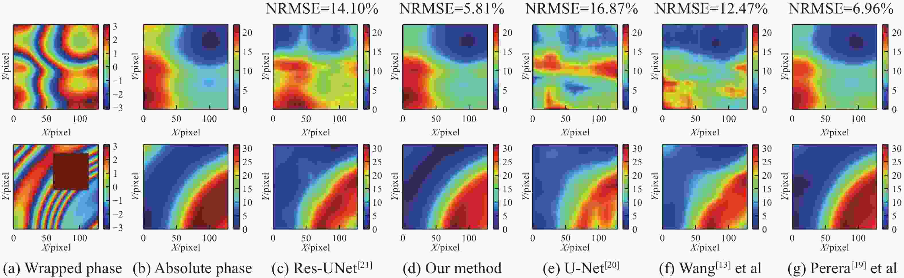
图  9  各个网络模型在真实数据集中的泛化能力

Figure 9.  The generalization ability of each network model in the real data set

1）噪声情况

图6分别显示了无噪声、轻微噪声、中度噪声、严重噪声、重度噪声五种情况，并依次加入高斯噪声，SNR分别为[0,5,10,20,80]。由此可以看出，在无噪声的情况下，五种网络模型均有一定的解包裹能力，但随着噪声的增加， Res-UNet^[21]和U-Net^[20]的性能都不太理想且耗时较长。在包裹相位中存在不同信噪比的噪声条件下，文中提出的网络均可以表现出色，不仅有最低的归一化均方根误差，还有达到收敛情况最少的训练次数。

2）不连续情况

从图7可以看出，在无噪声不连续情况下，五种网络模型的解包裹能力不同，文中提出的网络模型、Wang ^[13] 等人提出的网络和Perera^[19]提出的网络模型均有一定的解包裹能力，但是其他两种网络模型达到收敛需要较长时间。在不连续情况下，文中提出的网络表现出色，不仅有最低的归一化均方根误差，还有达到收敛情况最少的训练次数。

3）混叠情况

从图8可以看出，在同时存在噪声和不连续的情况下，五种网络模型的解包裹能力不同，文中提出的网络模型、Perera^[19]等人提出的网络模型在混叠情况下表现较好，且实验速度较快。在混叠情况下，文中提出的网络表现出色，不仅有最低的归一化均方根误差，还有达到收敛情况最少的训练次数。

4）泛化情况

图9用来验证用模拟数据集训练真实数据集验证网络解包裹性能的情况，由此可以看出，分别在噪声和不联系这两种不同的情况下，五种网络模型均有一定的模型泛化能力，但是均没有在模拟数据集中表现出色。其中，文中提出的网络依旧有很好的解包裹相位能力。

从图10可以看出，文中提出的相位解包裹技术在噪声(NRMSE =0.75%、SSIM=0.98、PSNR=40.87)、不连续(NRMSE=1.81%、SSIM=0.92、PSNR=32.56)、混叠(NRMSE =1.68%、SSIM=0.94、PSNR=37.38)三种不同情况下的性能优于其他网络，而且平均计算时间最低，模型达到收敛状态需要的平均训练轮次最少（153次）。

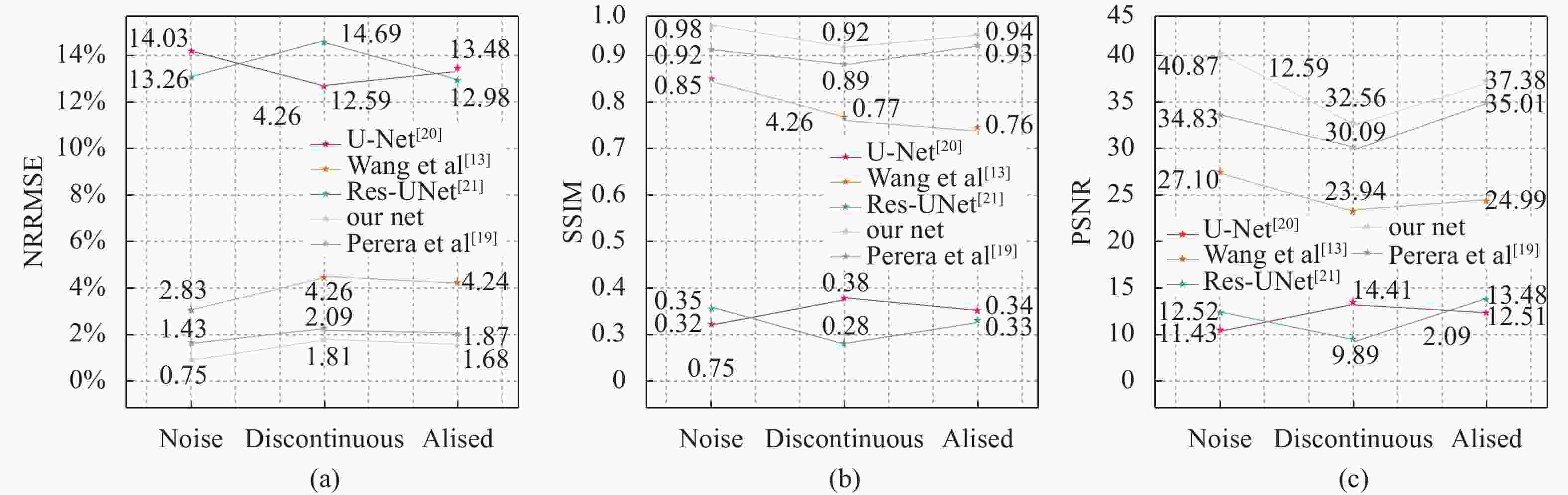
图  10  各个网络模型不同性能比较

Figure 10.  Different performance comparison of each network model

如表1和图10所示，相同的网络模型通过不同的损失函数进行训练会得到不同的结果。对于文中提出的网络，复合损失函数显然是比$ {L}_{mean} $和$ {L}_{error} $适合这个问题的损失函数。

此外，如表2、图10所示，在实验过程中，文中提出的网络受网络参数量增加的影响，每轮训练的时间慢于U-Net^[20]和Res-Net网络，但是达到最佳性能需要的轮数远小于其他网络，因此，当达到最佳收敛性能时，文中提出的网络所用时间最少。这些观察结果使笔者得出结论，所提出的网络的成功归功于CBiLSTM模块、注意力机制模块和复合损失函数。

图11展示了包裹相位经过文中提出的网络模型训练后输出的预测绝对相位与真实相位之间的比照，通过编码器-解码器模型的搭建、CBiLSTM模块与注意力机制模块的引入以及复合损失函数的定义，在与其他模型比较后，验证了文中提出的网络模型在前文提到的三种情况下在精度的提高与训练方面的减少。通过模拟实验的验证，通过增强深度学习模型对关键相位信息的关注能力，文中提出的网络模型能够提高相位解包裹的准确性和鲁棒性，推动光学测量和相位成像等领域的进一步发展。

图  11  文中提出的网络模型预测相位与真实绝对相位在上述三种情况下的对比

Figure 11.  Comparison between the predicted phase and the true absolute phase of the network model proposed in this article in the above three situations

文中采用基于改进U-Net网络的编码器-解码器架构，同时加入包含双向长短期记忆网络（BILSTM）的CBiLSTM模块，并且结合注意力机制，避免了典型卷积神经网络学习全局空间依赖关系的固有缺陷的同时增强了深度学习模型对相位解包裹任务中的关键信息的关注能力。为了验证CBiLSTM模块和注意力机制模块对单张图像解包裹产生的影响，下面进行消融实验。为了公平起见，下述实验都在随机噪声的包裹数据集上迭代了200次。实验的定量结果如表3所示。表中序号为1的模型表示为原始改进U-Net模型，实验结果表明，单纯地加入CBiLSTM模块或者注意力机制模块都对模型的性能产生积极影响，此外，同时加入CBiLSTM模块和注意力机制模块的模型与原模型和加入单一模块的模型相比表现出更加优秀的性能。

透射式光学偏折术通过显示屏幕显示设定的结构光，结构光通过光学透镜时发生折射，CCD相机采集到被光学透镜折射后的形变条纹图。通过对接收到的形变条纹包裹相位进行解包裹运算得到其绝对相位，其绝对相位各个点的相位斜率即可映射到透镜波前的梯度，进而反推波前形状。

相位解包裹是光学偏折术测量工作的重要组成成分。文中建立了一个实验测试系统，对一块球面透镜的表面进行测量，由于待测元件的光学性质，显示屏幕发出的光线在待测元件处发生光学偏折，借助第2节中提出的基于改进U-Net网络的模型，可以得到真实相位分布。测试系统由显示屏幕，CCD相机，待测透镜部分三部分组成，如图12所示。显示屏幕中心于CCD相机光轴在同一直线。

图  12  实验测试系统

Figure 12.  Experimental test system

实验中，将待测透镜夹持放置于显示屏幕和CCD相机中间，保证待测透镜的几何中心位于相机光轴，加入透镜后相机采集到的条纹图如图13所示。

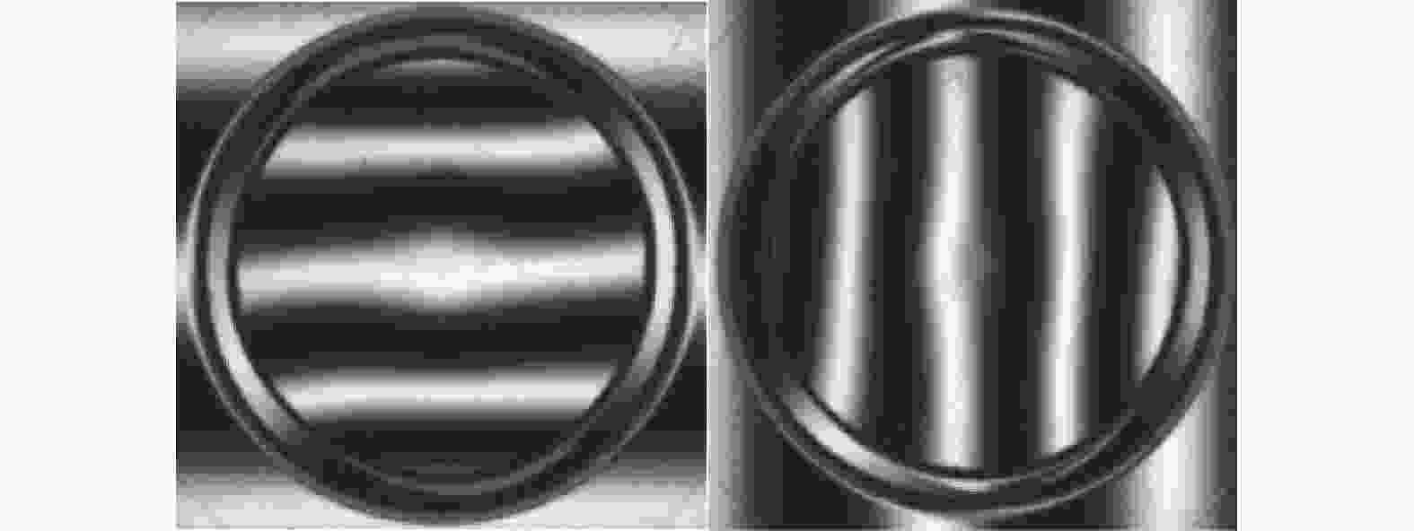
图  13  数据采集图

Figure 13.  Data acquisition diagram

使用第2节中叙述的相位解包裹模型对采集到的真实数据进行相位解包裹，可以得到的绝对相位图如图14所示，从实验结果来看，可以看出文中提出的网络在真实数据上仍然可以很好地工作。

图  14  真实数据集上的水平竖直方向的相位解包裹

Figure 14.  Horizontal and vertical phase unwrapping on real data sets

在实际测量中，相位解包裹的环境存在着各种意外情况，例如透镜表面的灰层等污点、透镜表面出现划痕等。这些因素可能导致相位数据中出现无效点，即不连续点的存在。这些无效点的存在会对相位解包裹算法的准确性和稳定性造成影响。因此，为了验证文中提出的相位解包裹算法在实际情况中的可靠性，下面用记号笔涂画模拟透镜存在灰尘和刮痕的情况，如图15所示。

图  15  透镜存在灰尘和划痕的实验情况图

Figure 15.  Picture of the experimental situation with dust and scratches on the lens

得到的包裹相位如图16（a）、（c）所示。通过对这些无效点的检测和处理，得到绝对相位如图16（b）、（d）所示。从实验结果来看，可以看出文中提出的网络在复杂真实数据上仍然可以很好地工作，文中提出的网络在真实复杂数据集中依旧具有可行性。

图  16  复杂真实数据集上的相位解包裹

Figure 16.  Phase unwrapping on complex real datasets

文中针对包裹相位展开问题，通过将其表述为回归问题，提出了一种新的卷积架构，该架构包含基于编码器-解码器架构的一系列改造，包括添加CBiLSTM模块，注意力机制模块等。与现有的几种相位展开方法进行比较，发现该网络在不需要大规模数据集训练的情况下，即使在严重噪声条件下、不连续、混叠等情况下也能获得较优秀的相位展开性能。此外，该网络执行此任务平均花费的计算时间显着减少，使其成为需要准确和快速相位展开任务的理想选择。同时在实验室真实数据集上面进行验证实验，发现该网络依旧有优秀的性能。文中提出的网络模型使传统方法无法解决的严重噪声、不连续与混叠情况下的相位解包裹任务变成可能，同时通过与其他深度学习模型的精度对比，归一化均方根误差低至0.75%。解包裹相位技术对光学自由曲面的检测意义非常重要，不仅体现在提高测量准确性、精确控制光学参数以及优化光学设计等方面，而且对于光学制造和检测的质量保证和性能提升具有重要作用。