


-
在光学系统的设计过程中,公差敏感度是决定设计是否优秀的一个重要因素。公差敏感度低的设计更有利于降低加工成本、简化装调流程,实现成像质量和生产良率的平衡[1]。为了得到公差不敏感的结构,往往需要在光学设计软件中进行迭代优化:可以通过全局优化[2]来获得大量样本,并直接从中寻找低公差敏感度的系统;或者通过建立多重结构[3]预先分配公差并建立综合评价函数来优化得到符合公差要求的结果。但这类方法缺乏光学理论的指导,重复、盲目的优化过程需要消耗大量的计算资源,效率较低。因此,为了提高优化效率,人们提出了多种降低公差敏感度的思路,并基于光学结构分析提出了多种评价参数。Betensky[4]将非球面应用于三片式镜头的设计中,避免负透镜承担过大的像差矫正压力,实现公差降敏;Ishiki[5]提出了针对光学表面偏折角控制的公差敏感度评价函数;Sasian[6]等提出了透镜形状特征参数W和S,并证明减小W、S值可实现良好的公差脱敏和像差平衡。此外,人们也尝试从像差入手,寻求针对特定像差进行优化度或是通过像差之间的相互补偿来实现公差敏感度的降低。Wang Lirong[7]提出了CS和AS评价函数用于对倾斜带来的恒定彗差和线性像散敏感度进行评价;张远健[8]等以均匀化各表面初级像差分布并抑制各表面初级像差贡献量为思路,提出了“小像差互补”的优化方法;刘智颖[9]等将其应用在红外显微系统设计中,取得了不错的效果;孟庆宇[10]等提出根据光学面与像面上光线交点的变化量计算得到相应的光程变化量,并将其作为公差灵敏度的评价标准;Sasian[11]利用波像差系数和结构参数总结了多种像差评价方法,并指出控制像差在光学系统内的传播可以有效降低公差敏感度。
然而,不同的光学系统具有各自的公差特性,为使公差优化具有更好的针对性,文中提出首先对引入像差进行定量分析,分析结果为评价函数和应用表面的设置提供指导,其目的是针对不同的引入像差降低其敏感度,进而提升优化效率。光学系统引入公差扰动后,直接导致成像质量降低。MTF、点列图等评价手段可以反映整个系统的像质表现,然而无法反映残余像差的组成;基于近轴光线追迹计算的Seidel系数可以反映初级像差的分布,但无法反映公差扰动后系统的像差特性。对于具有圆形孔径的光学系统,Zernike多项式给出了一组完备正交基,可以用于描述某一视场点处任意形状的波像差分布。同时,低阶 Zernike多项式系数与初级像差有着明确的对应关系[12],可以借此对光学系统的残余像差进行定量分析,找出光学系统扰动后引入的主要像差。
文中希望通过线性代数方法对轴对称光学系统引入公差后生成的新像差进行分析,确定主要的引入像差;基于节点像差理论(NAT)分析像差成因并给出用于抑制新像差生成的评价函数;最后通过实际光学系统的优化设计过程验证这一方法的有效性。
-
Zernike多项式给出了一套圆域上的正交基,可通过加权的离散面型项对波前进行拟合,是常用的波像差表达方式。利用Zernike多项式,系统的残余波像差可反映为多项线性叠加的形式,其中每一项都经过正则化,如公式(1)所示:
$$ \begin{array}{c}W\left(r,\theta \right)=\displaystyle\sum _{n,m} {Z}_{n}^{m}{R}_{n}^{m}\left(r,\theta \right)\end{array} $$ (1) 式中:W表示波像差;$ R $为Zernike项;$ Z $为对应系数;$ r $和$ \theta $为孔径坐标长度和方位角;n和m表示径向频率和角向频率。在高阶项很小的情形下,Zernike项与初级像差具有严格的对应关系[5]。因此,可以通过Zernike系数获知系统的像差分布,引入单位公差扰动后系数的变动即反映相应像差的敏感性。分析主要的敏感项将对降低公差敏感度提供指导作用。
在线性代数中,主成分分析 (Principal Component Analysis, PCA)可用于数据降维[13],其作用是将高维空间中的样本点信息(如利用Zernike多项式表述的波像差)投影在低维空间的坐标系中,通过计算数据矩阵中方差最大的几个投影方向即可获得新的低维坐标系。因此,该方法可用少数几个向量来表示完整的像差场分布。
对已有的理想结构进行Monte Carlo模拟,分析$ n $个扰动结构的前$ m $项Zernike系数相比初始结构的变化量,构成矩阵$ {D}_{m\times n} $:
$$ \begin{array}{c}{D}_{m\times n}=\left[\begin{array}{ccc}\Delta {Z}_{\mathrm{1,1}}& \cdots & {\Delta Z}_{1,n}\\ \vdots & \ddots & \vdots\\ {\Delta Z}_{m,1}& \cdots & {\Delta Z}_{m,n}\end{array}\right]\end{array} $$ (2) 为了找到方差最大的投影方向,首先求$ D $的协方差矩阵$ C $:
$$ \begin{array}{c}C=\dfrac{1}{n-1}\left(D-\overline{D}\right){\left(D-\overline{D}\right)}^{\prime}\end{array} $$ (3) 该协方差矩阵的特征值$ \tau $决定方差大小,即投影长度;特征向量$ p $决定了投影方向。将特征值由大到小排序,取显著偏大的前$ a $项特征值$ \tau $所对应的特征向量$ p $即可构成降维的像差空间。那么,添加扰动后系统的像差变化量可视为特征向量$ p $的线性组合,表示为:
$$ \begin{array}{c}{\Delta Z}_{m\times 1}=\displaystyle\sum _{s=1}^{a}{k}_{s}{p}_{s}\end{array} $$ (4) 式中:$ {k}_{s} $为常数。这些特征向量$ p $构成了一个新的像差空间,其中的每一项都与Zernike系数相对应,即$ {p}_{s}\left(i\right)={\Delta Z}_{i,s} $。其中,显著偏大的项反映了该投影方向在原像差空间中的主要分量(即主要的Zernike项),因此揭示了主要的引入像差。此外,PCA可以解除线性相关,将不同类别的像差归入不同的向量$ p $中,这可以揭示像差之间的耦合关系。
-
基于上述分析的结果,下面将讨论如何从像差分析的角度对引入像差进行控制。光学系统波像差可由一个与视场和孔径位置相关的函数来表达。对于旋转对称的光学系统,利用视场坐标$ \overrightarrow{H} $、光曈坐标$ \overrightarrow{\rho } $以及两个矢量方位角的夹角$ \theta $即可唯一地确定一条光线。此外,这里将轻微扰动的光学系统视为线性系统,总像差可以看作各个表面像差贡献量之和。基于以上概念,Hopkins[14]提出了标量波像差表达式:
$$\begin{split} & W\left(H,\rho ,\theta \right)=\displaystyle\sum _{q,m,n} {W}_{k,l,m}{H}^{2q+m}\cdot {\rho }^{2n+m}\cdot {\cos}^{m}\theta \\&\qquad\qquad k=2q+m,l=2n+m \end{split}$$ (5) 式中:$ W $为像差系数,$ q $、$n、m$为整数,根据视场和孔径的幂次确定。
在此基础上,为了描述光学表面经过偏心、倾斜等扰动而产生失对称的光学系统的像差特性,Buchroeder[15]、Shack和Thompson[16]在1980年提出了节点像差理论。偏心、倾斜等公差扰动会造成局部像差场的偏移,而节点像差理论将像面与光瞳面视为二维向量空间,因此可以方便地引入局部像差场偏移量$ \overrightarrow{\sigma } $。引入扰动$ \overrightarrow{\sigma } $后的像差场可描述为:
$$ \begin{split} & W\left(\overrightarrow{H},\overrightarrow{\rho }\right)=\displaystyle\sum _{i} \sum _{q,m,n} {W}_{q,m,n}{\left(\left(\overrightarrow{H}-{\overrightarrow{\sigma }}_{i}\right)\cdot \left(\overrightarrow{H}-{\overrightarrow{\sigma }}_{i}\right)\right)}^{q}\cdot\\&\qquad\qquad {\left(\left(\overrightarrow{H}-{\overrightarrow{\sigma }}_{i}\right)\cdot \overrightarrow{\rho }\right)}^{m}\cdot {\left(\overrightarrow{\rho }\cdot \overrightarrow{\rho }\right)}^{n} \end{split}$$ (6) 式中:i为表面序号。光学表面经失对称扰动的模型如图1所示。

图 1 失对称扰动模型
Figure 1. Asymmetric perturbation model
在光学装调的过程中,偏心仪采用球心像相对光轴的偏离来检测偏心、表面倾斜等加工误差。这里采用表面曲率中心的偏移来反映光学面的偏心和倾斜程度,根据文献[17],可用偏移角$ \beta $来表示,它是球心偏移量$ \Delta c $与表面曲率半径$ R $之比。
$$ \begin{array}{c}\beta =\dfrac{\Delta c}{R}\end{array} $$ (7) 根据Thompson的推导[17],偏移量$ \sigma $的大小取决于零视场处主光线角$ {\varphi }_{OAC} $与偏移角$ \beta $之差与边缘视场主光线入射角$ {\varphi }_{MC} $之比。在灵敏度分析中,不同表面和元件的不同误差往往分开考虑,一次只分析一个对象的扰动。因此,这里不考虑由前序表面带来的视场和光曈偏移,主光线和边缘光线按理想情况追迹,此时对于同轴光学系统,$ {\varphi }_{OAC} $=0。综上,偏移量$ \sigma $的计算公式可简化为:
$$ \begin{array}{c}\sigma =\dfrac{\beta }{{\varphi }_{MC}}\end{array} $$ (8) 基于节点像差理论,可以从现有理想结构中推断出可能的引入像差及其影响。由公式(6)可知,扰动量$ \overrightarrow{\sigma } $的引入带来了新的像差项,根据新产生项的视场与孔径相关性可以推断产生的像差类型[18]。表1列出了几种引入像差的表达式。
表 1 部分引入像差类型
Table 1. Several types of induced aberration
Induced aberration Mathematical expression Tilt $ {W}_{111}\left(\overrightarrow{\sigma }\cdot \overrightarrow{\rho }\right)={W}_{111}\sigma \rho \mathrm{c}\mathrm{o}\mathrm{s}\theta $ Uniform coma $ {W}_{131}(\overrightarrow{\sigma }\cdot \overrightarrow{\rho })(\overrightarrow{\rho }\cdot \overrightarrow{\rho })={W}_{131}\sigma {\rho }^{3}\mathrm{c}\mathrm{o}\mathrm{s}\theta $ Linear astigmatism $ {W}_{222}(\overrightarrow{\sigma }\cdot \overrightarrow{\rho })(\overrightarrow{H}\cdot \overrightarrow{\rho })={W}_{222}\sigma H{\rho }^{2}{\mathrm{c}\mathrm{o}\mathrm{s}}^{2}\theta $ Uniform astigmatism $ {W}_{222}(\overrightarrow{\sigma }\cdot \overrightarrow{\rho })(\overrightarrow{\sigma }\cdot \overrightarrow{\rho })={W}_{222}{\sigma }^{2}{\rho }^{2}{\mathrm{c}\mathrm{o}\mathrm{s}}^{2}\theta $ 其中,$ W $和$ \sigma $可通过追迹轴上视场边缘光线和边缘视场主光线计算得到,这意味着可以在理想结构优化过程中经由光线追迹结果快速计算得到引入像差,无需进行额外的统计分析。
综上所述,失对称公差引起的像差可视为以上项的线性叠加:
$$ \begin{split} &\quad {W}_{dl}={W}_{111}\left(\overrightarrow{\sigma }\cdot \overrightarrow{\rho }\right)+{W}_{131}\left(\overrightarrow{\sigma }\cdot \overrightarrow{\rho }\right)\left(\overrightarrow{\rho }\cdot \overrightarrow{\rho }\right)+\\& {W}_{222}\left(\overrightarrow{\sigma }\cdot \overrightarrow{\rho }\right)\left(\overrightarrow{H}\cdot \overrightarrow{\rho }\right)+{W}_{222}\left(\overrightarrow{\sigma }\cdot \overrightarrow{\rho }\right)\left(\overrightarrow{\sigma }\cdot \overrightarrow{\rho }\right)+\cdots \end{split} $$ (9) -
节点像差理论可以通过引入视场偏移矢量来描述由偏心、倾斜等造成光学系统失对称的扰动所带来的像差。然而,对于厚度、空气间隔等轴向扰动所带来的成像质量损失,并不会造成光瞳坐标$ \rho $或视场坐标$ H $的位移。在高数值孔径等边缘光线角度较大的情形中,厚度改变会导致不同孔径处光程的差异,带来了像差场的变化。对于波像差敏感的高分辨率光学系统,这可能造成成像质量的严重下降[19],且如果在偏心、倾斜等扰动同时存在且镜片数目较多的情形下,情况将更为复杂,可能会导致轴外像差场的改变。此时采用空气间隔补偿不足以起到良好的效果,因此对轴向扰动引起的像差进行抑制同样重要。
为了简化分析,这里仅对轴上视场点且光学表面为球面的情况进行分析。表面轴向扰动$ \Delta t $后,边缘光线入射高度变化$ \Delta y $,如图2所示。这种变化会引入新的波像差项$ {W}_{t} $。这里将材料折射率公差也视为一种轴向扰动,因为它同样造成了光程变化$ {W}_{i}=\Delta n\cdot t $,$ t $为该光线经过的介质厚度。同时,$ {W}_{dm} $可以视为视场无关的新增波像差的线性组合,由公式(6)可得:
$$ {W}_{dm}={W}_{t}+{W}_{i} =\Delta {W}_{020}\left(\overrightarrow{\rho }\cdot \overrightarrow{\rho }\right)+\Delta {W}_{040}\text{}{\left(\overrightarrow{\rho }\cdot \overrightarrow{\rho }\right)}^{2}+\cdots $$ (10) 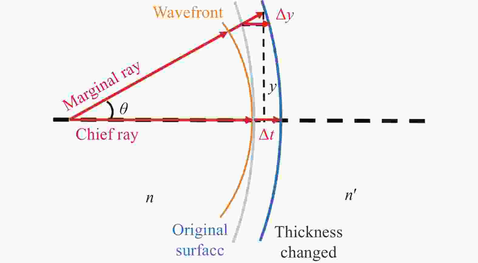
图 2 轴向扰动模型
Figure 2. Axial perturbation model
其中,$ \Delta {W}_{020} $和$ \Delta {W}_{040} $由离焦和球差波像差系数关于$ y $求导得到:
$$ \Delta {W}_{020}=\Delta y\left(A^{\prime}-A\right) $$ $$ \begin{array}{c}\Delta {W}_{040}=-\dfrac{1}{4}\Delta y{A}^{2}\left(\dfrac{{u}^{\prime}}{{n}^{\prime}}-\dfrac{u}{n}\right)\end{array} $$ (11) $$ \Delta y=\Delta t\cdot {\rm{tan}}(-u) $$ 式中:$A=ni;A^{\prime}=n^{\prime}i^{\prime}$,为光线在表面折射前后的阿贝不变量;$ u $为边缘光线角。
-
以上分析表明,公差扰动会导致新像差项的产生。建立起相应的评价函数,在设计阶段对公差扰动引起的新像差的产生进行估计并纳入优化,即可实现公差灵敏度的降低。
对于引起系统失对称的公差扰动,新生成的像差如表1所示。由于实际光线追迹中归一化的视场向量和光瞳向量的选取具有任意性,这里选择两向量长度为1且夹角$ \theta $为0时的情形构建评价函数。评价函数中的每一项对应着一种引入像差,其权重$ e $由PCA分析得到的特征值$ {\tau }_{s} $和特征向量$ {p}_{s} $的数值大小共同决定,其余部分代表由单位扰动$ \sigma $造成的引入像差。对于第$ i $面,失对称扰动评价函数可设置为:
$$ \begin{split} {m}_{offaxis,i}=&{{e}_{111}W}_{111,i}{\sigma }_{i}+{{e}_{131}W}_{131,i}{\sigma }_{i}+\\& {e}_{222}{W}_{222}\left({\sigma }_{i}+{{\sigma }_{i}}^{2}\right)+\cdots \end{split} $$ (12) 同理,对于轴向公差扰动:
$$ {m}_{onaxis,i}={e}_{020}\Delta {W}_{020}+{e}_{222}\Delta {W}_{040}+\cdots $$ (13) 系统的评价函数$ M $:
$$ \begin{array}{c}M=\displaystyle\sum _{i}{m}_{offaxis,i}+{m}_{onaxis,i}\end{array} $$ (14) 这里考虑到Zernike项中存在像差耦合,Zernike系数对应项与波像差系数对应项的光曈阶数不完全一致,因此将特征向量$ {p}_{s} $构成的以Zernike系数表达的向量空间转换为由像差权重因子$ e $表示的一维向量空间。根据波像差对应的光曈向量阶数,权重因子$ e $可设置为:
$$ \begin{array}{c}{e}_{111}=\displaystyle\sum _{s=1}^{a}{\tau }_{s}\left(\genfrac{}{}{0pt}{}{{p}_{s}\left(2\right)-2{p}_{s}\left(7\right)}{{p}_{s}\left(3\right)-2{p}_{s}\left(8\right)}\right)\end{array} $$ (15) $$ \begin{array}{c}{e}_{020}=\displaystyle\sum _{s=1}^{a}{\tau }_{s}\left(2{p}_{s}\left(4\right)-6{p}_{s}\left(9\right)\right)\end{array} $$ (16) $$ \begin{array}{c}{e}_{131}=\displaystyle\sum _{s=1}^{a}{\tau }_{s}\left(\genfrac{}{}{0pt}{}{3{p}_{s}\left(7\right)}{3{p}_{s}\left(8\right)}\right)\end{array} $$ (17) $$ \begin{array}{c}{e}_{040}=\displaystyle\sum _{s=1}^{a}{\tau }_{s}\left(6{p}_{s}\left(9\right)\right)\end{array} $$ (18) 式中:$ {p}_{s} $为公式(4)中提到的特征向量。从像差空间的角度考虑,权重因子的意义在于反映了添加扰动后系统像差的变化“方向”(趋势),而变化的“长度”则由权重因子和单位扰动造成的引入像差共同决定。利用光学设计软件将评价函数纳入优化计算流程中进行迭代优化,即可获得公差不敏感的结构。根据PCA分析的结果,可以灵活地调整$ M $中的项数以及更改评价函数所应用的表面,进行迭代优化,最终获得公差灵敏度符合要求的结构。上述分析和优化流程如图3所示。

图 3 公差降敏流程
Figure 3. Workflow of tolerance sensitivity reduction
-
基于上述理论分析,以两个系统为例来阐释整个工作流程,并验证该方法的有效性。第一个例子系统参数如表2所示。
表 2 结构1系统参数
Table 2. System parameters of Structure 1
Parameter Value Working F# 11 Magnification 1.35× EFL/mm 94 Wavelength/nm 460-635 该系统像质表现良好,MTF性能接近衍射极限,其结构如图4所示。

图 4 结构1二维图
Figure 4. Layout of Structure 1
对其进行灵敏度分析,以后截距作为补偿器,波前RMS值作为评价指标。公差扰动量设置及优化前后结果如表3所示。
表 3 结构1公差设置及优化前后结果 (MTF @36 lp/mm,轴上视场)
Table 3. Tolerance setting and performance of Structure 1 (36 lp/mm@ MTF, on-axis)
Parameter Value Thickness ±0.02 mm Surface radius ±3 fringes Surface tilt ±1' Element decenter ±0.015 mm Element tilt ±1' Nominal Mean Standard deviation Original 0.701 0.347 0.120 Optimized 0.687 0.505 0.082 灵敏度分析结果显示,前10个敏感项中主要包括第4片的偏心与第13面的表面倾斜。对该结构运行Monte Carlo分析,统计1000个样本结构的MTF在36 lp/mm处的原始值、平均值以及标准差,结果如表3所示。
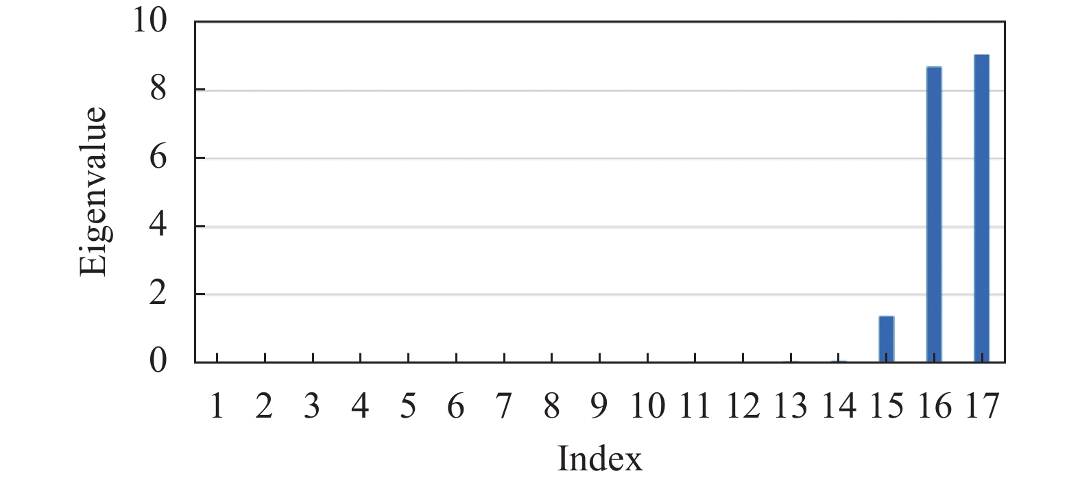
为了了解该系统引入公差后的像差特性,首先对其进行一次Monte Carlo分析,统计1000个结构相比初始结构的Zernike系数变化量。这里取前17项Zernike系数构成公式(3)中的矩阵D。根据1.1节中提到的方法,求取协方差矩阵C的特征值和特征向量。对特征值τ由小到大进行排序,如图5所示。

图 5 特征值分布
Figure 5. Distribution of eigenvalues
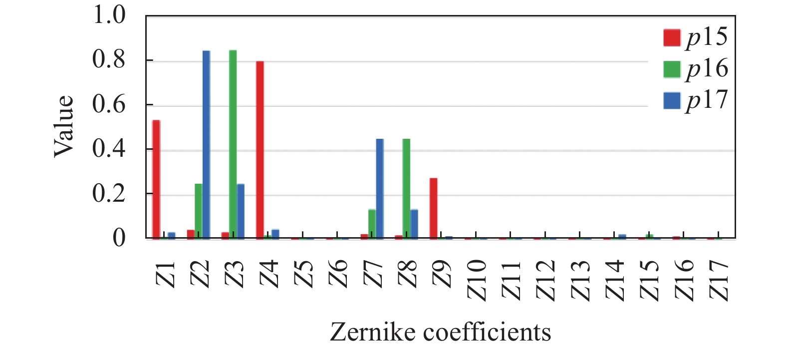
由图5可见,15、16、17三项特征值显著大于其余各项,因此取其对应的三个特征向量进行线性组合即可表征系统残余像差的特性,这三个特征向量中的每个元素都与Zernike系数Z相对应。三个向量中系数值的分布如图6所示。

图 6 主要特征向量的Zernike系数分布
Figure 6. Zernike coefficients distribution of main eigenvectors
基于文献[8]中建立的Zernike系数与像差的对应关系进行分析,系数Z9~Z17项很小,这意味着公差扰动主要造成初级像差的产生。可以看出,向量$ {p}_{15} $主要表现了引入的轴向像差,包括位移、离焦和球差。而$ {p}_{16} $和$ {p}_{17} $具有“对称”的分布,其中主要包含引入的$ x $和$ y $方向的倾斜以及彗差。计算系统引入像差的权重分布,可知该系统中主要引入像差是由失对称扰动引起的彗差,如图7所示。

图 7 结构1不同引入像差的权重分布
Figure 7. Weight distribution of induced aberrations in Structure 1
对各面的引入彗差进行计算,找出引入彗差的主要来源表面。这里设$ \Delta c=0.02 $ mm,各面的引入彗差$ {W}_{131,i}{\sigma }_{i} $分布如图8所示。可以看到,表面13具有最大的引入彗差,这与之前灵敏度分析的结果吻合。因此,这里对彗差贡献量较大的表面4、7、13设置只包含引入彗差项的评价函数M,进行全局优化。从图8中可以看出,优化后主要敏感面的引入彗差有所下降,并且总引入量绝对值更小。得到的结构如图4(b)所示,对该结构同样进行一次Monte Carlo分析,结果如表3所示。该结构像质较初始结构略有下降,但是公差灵敏度更低,因此引入公差后的估计性能表现更好。各视场优化前后的MTF表现如图9所示,其中红色线为优化后结果,蓝色线为优化前结果。可以看到,优化后系统的制造良率显著提升,以轴上视场为例,36 lp/mm处98%置信度的MTF性能相比优化前提升了68%。
以上优化基于笔者使用的笔记本电脑(AMD R7-5800 CPU, 16 GB DDR4 RAM),优化时间为36 min。这里使用Zemax软件中内嵌的TOLR操作数,将灵敏度分析的前10项作为公差编辑器参数进行优化。优化7 h后,轴上视场处98%结构在36 lp/mm处的MTF值大于$ 0.41 $,与图9中该方法优化后的结果相似。对比可见,该方法通过对特定像差和表面针对性地设置优化函数,可以实现公差灵敏度的有效降低,并且节省了大量优化时间。

图 8 不同表面引入彗差的分布
Figure 8. Distribution of induced coma on different surfaces
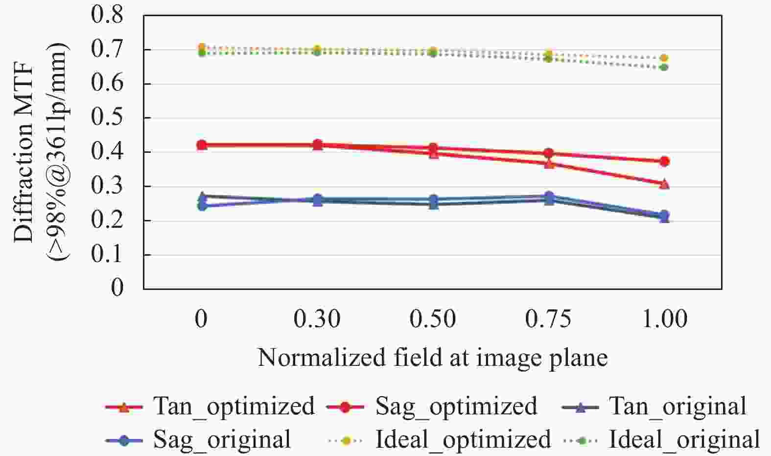
图 9 结构1优化前后MTF表现(>98% MTF@36 lp/mm)
Figure 9. MTF performance before and after optimization of Structure 1 (>98% MTF@36 lp/mm)
在第二个例子中,尝试利用该方法降低一个更为复杂的高数值孔径光学系统的公差灵敏度,系统参数如表4所示。该系统的公差特点在于它不止对失对称扰动公差敏感,轴向扰动也会带来明显的成像质量损失,系统初始结构如图10(a)所示。以表5中的设置对其进行灵敏度分析,发现第1、7、8镜片的厚度是敏感的公差项。

图 10 结构2二维图
Figure 10. Layout of Structure 2
表 4 结构2系统参数
Table 4. System parameters of Structure 2
Parameter Value NA 0.5 Magnification 5× Total length/mm 110 Wavelength/nm 460-635 表 5 结构2公差设置及优化前后结果 (MTF@180 lp/mm,轴上视场)
Table 5. Tolerance setting and nominal performance of Structure 2 (180 lp/mm@ MTF, on-axis)
Parameter Value Thickness ±0.01 mm Surface radius ±1 fringes Surface tilt ±1' Element decenter ±0.01 mm Element tilt ±1' Nominal Mean Standard deviation Original 0.345 0.243 0.075 Optimized 0.327 0.272 0.066 如图11所示,对结构2进行PCA分析,发现球差权重因子$ {e}_{040} $相比结构1明显更大,这意味着虽然引入扰动后系统的新增像差趋势依旧是彗差占主导地位,但球差的影响更加显著,以至于不能忽略。

图 11 结构2不同引入像差的权重分布
Figure 11. Weight distribution of induced aberrations in Structure 2
分析不同玻璃和空气间隔处轴向扰动造成的轴向像差,敏感项的分布与灵敏度分析结果吻合。对相应表面设置评价函数$ M $进行全局优化,优化前后引入像差分布如图12所示。可以看到,优化后大部分表面引入像差降低,总引入像差也略有下降。对优化后的结构进行一次Monte Carlo分析,结果如表5所示。结果显示,对于轴上视场,优化后90%的结构在180 lp/mm处的MTF值大于$ 0.167 $,相比优化前提升了约20%,如图13所示。作为对比,同样使用Zemax中的TOLR操作数进行优化,在运行7 h后,评价函数未出现变化,因此未能成功实现该结构的公差降敏。可见,该方法对于复杂结构的轴向扰动公差同样具有良好的降敏作用。

图 12 不同表面引入轴向像差的分布
Figure 12. Distribution of induced axial aberration on different surfaces
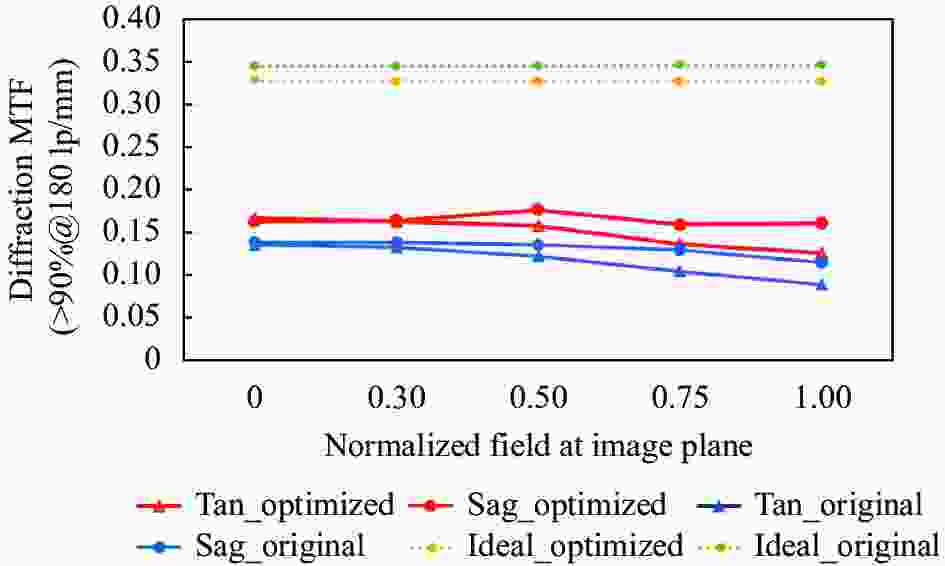
图 13 结构2优化前后MTF表现(>90% MTF@180 lp/mm)
Figure 13. MTF performance of Structure 2 (>90% MTF@180 lp/mm)
-
文中提出了一种基于引入像差分析和抑制的公差灵敏度降低方法。通过线性代数的方法对引入像差的类型和变化趋势进行统计分析,找出主要的引入像差。之后,针对失对称扰动和轴向扰动进行分析,利用节点像差理论对新生成像差进行预测,分析结果与传统灵敏度分析结果吻合。基于以上分析,提出了一个新颖的评价函数M,该评价函数以公差分析为依据对不同镜头进行有针对性的设置,并且通过两个光学系统的优化过程验证了它的有效性。其中,结构1优化后的性能相比优化前提升了约68%,实现同样优化效果的优化时间缩减为使用TOLR操作数时的1/14;对于更为复杂的结构2,该方法依然能够成功实现降敏。优化结果表明,该方法可以在节省计算资源的同时有效降低公差灵敏度。
Tolerance desensitization method based on principal component analysis and nodal aberration theory
-
摘要: 为了在设计阶段预测光学系统加工装配后的像质并降低加工装配难度,提升设计效率,文中提供了一个高效的公差灵敏度降低方法。首先使用Zernike多项式量化像差,基于线性代数理论和Monte Carlo分析寻找引入扰动后系统的像差变化规律,通过降维后的像差场以及特征值分布确定主要引入像差;对系统制造过程中可能出现的失对称扰动和轴向扰动进行建模,基于节点像差理论描述扰动造成的引入像差,并通过统计分析确定关键表面;根据Zernike项与波像差的对应关系对像差空间进行变换,提出相应的评价函数纳入优化,进而抑制新像差的产生。将这一方法应用于两个不同的光学系统的设计,优化后预期加工性能(指定空间频率处98%置信度的MTF表现)分别提升了约68%和20%。与使用Zemax软件中TOLR操作数优化相比,结构1的优化时间由7 h缩短到36 min,并且在结构2的优化中成功实现了公差降敏。结果表明,该方法能够在提升效率的同时有效降低公差灵敏度。Abstract:
Objective Optical systems with low tolerance sensitivity have good machinability and high manufacturing yield, reducing processing and adjustment costs. To achieve this, it is necessary to evaluate and optimize the system's tolerance sensitivity in its design, so it is necessary to study related desensitization methods. Traditional desensitization methods include using global optimization algorithms, establishing multiple structures or a combination of both to conduct extensive searches in the solution space, which requires a large amount of computational resources and has low optimization efficiency. Besides, the method by controlling the system structure and ray tracing parameters (such as surface curvature, ray deflection angle, etc.) or optimizing specific aberration distributions to obtain tolerance-insensitive structures lacks the analysis of introduced aberrations, and there is still a certain blindness in the setting of evaluation functions, which also affects the optimization efficiency. Therefore, in order to achieve higher optimization efficiency, this paper proposes a tolerance desensitization method based on the analysis and control of introduced aberrations, and provides corresponding operation counts. Methods Zernike polynomials are used to quantify aberrations. Based on this, linear algebra theory and Monte Carlo analysis are used to find the aberration change rule of the system after introducing perturbations. The main introduced aberrations are then determined through the aberration field and eigenvalue distribution after dimension reduction (Fig.7, Fig.11). Asymmetric perturbations and axial perturbations that may occur during the system manufacturing process are modeled. The introduced aberrations caused by the perturbations are described based on the node aberration theory, and the key surfaces are determined through statistical analysis (Fig.8, Fig.12). According to the correspondence between Zernike terms and wave aberrations, the aberration space is transformed, and a corresponding evaluation function is proposed. Based on the previous analysis, the weights and application surfaces of each term of the evaluation function are determined, and then it is included in the optimization process to suppress the generation of new aberrations. The analysis and optimization ideas of this method are shown (Fig.3). Results and Discussions This method has been applied to the design of the F#11 optical system (Structure 1) and the NA0.5 optical system (Structure 2). After optimization, the expected machining performance has been significantly improved. Taking the MTF performance at the specified spatial frequency on the axis with a 98% confidence level as an example, the performance of the two systems after optimization has increased by about 68% (Fig.9) and 20% (Fig.13) respectively. Compared with the optimization using the TOLR operation number in Zemax software, the optimization time of Structure 1 has been reduced from 7 hours to 36 minutes, and tolerance desensitization has been successfully achieved in the optimization of Structure 2. Conclusions A method for reducing tolerance sensitivity based on the analysis and suppression of introduced aberrations is proposed. The obtained Zernike coefficient matrix is processed by the method of principal component analysis, and the dimensionality reduction of the aberration space is realized according to the obtained eigenvalues and their corresponding eigenvectors. After analyzing the dimensionally reduced aberration space, the main introduced aberration items after perturbation are clarified. The types of aberrations caused by asymmetric perturbations and axial perturbations in the optical system are analyzed, and the quantitative expression of the introduced aberration items is obtained based on the node aberration theory. According to the correspondence between Zernike terms and primary aberrations, the expression of the evaluation function M is derived. The evaluation function is applied to two design examples, and the optimization results show that this method has higher optimization efficiency compared to existing methods, and it has a tolerance desensitization effect on optical systems with different complexities and different introduced aberration characteristics. -
图 6 主要特征向量的Zernike系数分布
Figure 6. Zernike coefficients distribution of main eigenvectors
图 7 结构1不同引入像差的权重分布
Figure 7. Weight distribution of induced aberrations in Structure 1
图 9 结构1优化前后MTF表现(>98% MTF@36 lp/mm)
Figure 9. MTF performance before and after optimization of Structure 1 (>98% MTF@36 lp/mm)
图 11 结构2不同引入像差的权重分布
Figure 11. Weight distribution of induced aberrations in Structure 2
图 12 不同表面引入轴向像差的分布
Figure 12. Distribution of induced axial aberration on different surfaces
图 13 结构2优化前后MTF表现(>90% MTF@180 lp/mm)
Figure 13. MTF performance of Structure 2 (>90% MTF@180 lp/mm)
表 1 部分引入像差类型
Table 1. Several types of induced aberration
Induced aberration Mathematical expression Tilt $ {W}_{111}\left(\overrightarrow{\sigma }\cdot \overrightarrow{\rho }\right)={W}_{111}\sigma \rho \mathrm{c}\mathrm{o}\mathrm{s}\theta $ Uniform coma $ {W}_{131}(\overrightarrow{\sigma }\cdot \overrightarrow{\rho })(\overrightarrow{\rho }\cdot \overrightarrow{\rho })={W}_{131}\sigma {\rho }^{3}\mathrm{c}\mathrm{o}\mathrm{s}\theta $ Linear astigmatism $ {W}_{222}(\overrightarrow{\sigma }\cdot \overrightarrow{\rho })(\overrightarrow{H}\cdot \overrightarrow{\rho })={W}_{222}\sigma H{\rho }^{2}{\mathrm{c}\mathrm{o}\mathrm{s}}^{2}\theta $ Uniform astigmatism $ {W}_{222}(\overrightarrow{\sigma }\cdot \overrightarrow{\rho })(\overrightarrow{\sigma }\cdot \overrightarrow{\rho })={W}_{222}{\sigma }^{2}{\rho }^{2}{\mathrm{c}\mathrm{o}\mathrm{s}}^{2}\theta $  下载: 导出CSV
表 2 结构1系统参数
Table 2. System parameters of Structure 1
Parameter Value Working F# 11 Magnification 1.35× EFL/mm 94 Wavelength/nm 460-635
下载: 导出CSV
表 3 结构1公差设置及优化前后结果 (MTF @36 lp/mm,轴上视场)
Table 3. Tolerance setting and performance of Structure 1 (36 lp/mm@ MTF, on-axis)
Parameter Value Thickness ±0.02 mm Surface radius ±3 fringes Surface tilt ±1' Element decenter ±0.015 mm Element tilt ±1' Nominal Mean Standard deviation Original 0.701 0.347 0.120 Optimized 0.687 0.505 0.082
下载: 导出CSV
表 4 结构2系统参数
Table 4. System parameters of Structure 2
Parameter Value NA 0.5 Magnification 5× Total length/mm 110 Wavelength/nm 460-635
下载: 导出CSV
表 5 结构2公差设置及优化前后结果 (MTF@180 lp/mm,轴上视场)
Table 5. Tolerance setting and nominal performance of Structure 2 (180 lp/mm@ MTF, on-axis)
Parameter Value Thickness ±0.01 mm Surface radius ±1 fringes Surface tilt ±1' Element decenter ±0.01 mm Element tilt ±1' Nominal Mean Standard deviation Original 0.345 0.243 0.075 Optimized 0.327 0.272 0.066
下载: 导出CSV
-
[1] 任成明, 孟庆宇, 秦子长 . 大型自由曲面离轴三反光学系统降敏设计(特邀) [J]. 红外与激光工程,2023 ,52 (7 ):20230287 . doi: 10.3788/IRLA20230287 Ren Chengming, Meng Qingyu, Qin Zichang. Desensitization design of large freeform off-axis three-mirror optical system ( invited) [J]. Infrared and Laser Engineering, 2023, 52(7): 20230287. (in Chinese) doi: 10.3788/IRLA20230287[2] Kuper T, Harris T. A new look at global optimization for optical design [J]. Photonics Spectra, 1992, 1: 151-160. [3] Fuse K. Method for designing a refractive optical system and method for designing a diffraction optical element: US, 6567226[P]. 2002-05-20. [4] Betensky E I. Aberration correction and desensitization of an inverse-triplet object lens [C]//Proceedings of SPIE, 1998, 3482: 264-268. doi: 10.1117/12.322011 [5] Isshiki M, Sinclair D C, Kaneko S. Lens design: global optimization of both performance and tolerance sensitivity [C]//Proceedings of SPIE, 2006, 6342: 63420N. [6] Sasian J M, Descour M R. Power distribution and symmetry in lens systems [J]. Optical Engineering, 1998, 37(3): 1001-1004. doi: 10.1117/1.601933 [7] Wang L R, Sasian J M. Merit figures for fast estimating tolerance sensitivity in lens systems [C]//Proceedings of SPIE, 2010, 7652: 76521P. doi: 10.1117/12.868874 [8] 张远健, 唐勇, 王鹏, 等 . 光学系统设计中降低公差灵敏度的方法 [J]. 光电工程,2011 ,38 (10 ):127 -133 . Zhang Y J, Tang Y, Wang P, et al. Method of tolerance sensitivity reduction of optical system design [J]. Opto-Electronic Engineering, 2011, 38(10): 127-133.[9] 刘智颖, 吕知洋, 高柳絮 . 红外显微光学系统的小像差互补设计方法 [J]. 红外与激光工程,2021 ,50 (2 ):20200153 . doi: 10.3788/IRLA20200153 Liu Zhiying, Lv Zhiyang, Gao Liuxu. Design method of infrared microscope optical system with lower aberration compensation [J]. Infrared and Laser Engineering, 2021, 50(2): 20200153. (in Chinese) doi: 10.3788/IRLA20200153[10] Meng Q, Wang H, Wang W. Sensitivity theoretical analysis and desensitization design method for reflective optical system based on optical path variation[J]. Opt Precis Eng. 2021, 29, 72–83. 孟庆宇, 汪洪源, 王维等. 基于光程变化量的反射式光学系统敏感度理论分析与降敏设计方法[J]. 光学精密工程, 2021, 29(01): 72-83. Meng Qingyu, Wang Hongyuan, Wang Wei, et al. Sensitivity theoretical analysis and desensitization design method for reflective optical system based on optical path variation[J]. Opt Precis Eng , 2021, 29(1): 72–83. (in Chinese) [11] Sasian J M. Lens desensitizing: theory and practice [J]. Applied Optics, 2022, 61(3): A62-A67. doi: 10.1364/AO.443758 [12] Gross H. Handbook of Optical Systems: Vol. 3. Aberration Theory and Correction of Optical Systems[M]. US: John Wiley & Sons, 2007: 56. [13] Jain P. Optical tolerancing and principal component analysis [J]. Applied Optics, 2015, 54(6): 1439-1442. doi: 10.1364/AO.54.001439 [14] Hopkins H H. Wave Theory of Aberrations[M]. Oxford: Clarendon Press, 1950. [15] Buchroeder R A. Tilted component optical systems[D]. Tucson: University of Arizona, 1976. [16] Shack R V, Thompson K. Influence of alignment errors of a telescope system on its aberration field [C]//Proceedings of SPIE, 1979, 251: 146-153. [17] Thompson K P, et al. Real-ray-based method for locating individual surface aberration field centers in imaging optical systems without rotational symmetry [J]. Journal of the Optical Society of America A, 2009, 26(6): 1503-1517. doi: 10.1364/JOSAA.26.001503 [18] Bauman B J, Schneider M D. Design of optical systems that maximize as-built performance using tolerance/compensator-informed optimization [J]. Optics Express, 2018, 26(11): 13819-40. doi: 10.1364/OE.26.013819 [19] 白晓泉, 郭良, 马宏财, 许博谦, 鞠国浩, 徐抒岩 . 离轴三反望远镜轴向与横向失调量像差耦合特性 [J]. 中国光学,2022 ,15 (4 ):747 -60 . Bai Xiaoquan, Guo Liang, Ma Hongcai, et al. Aberration coupling characteristics of axial and lateral misalignments of off-axis three-mirror telescopes [J]. Chinese Optics, 2022, 15(4): 747-760. (in Chinese) -

 点击查看大图

计量
- 文章访问数: 108
- HTML全文浏览量: 29
- PDF下载量: 31
- 被引次数: 0

