海洋水体的光学特性参数的剖面探测对海洋资源管理、海洋生态环境安全、水质生态监测、海洋研究等领域具有重要意义^[1]。目前常用的海洋探测手段包括原位探测、被动探测和主动探测。原位探测技术^[2]通过单点测量方式获取水体参数的剖面信息，其数据的准确性较高，常作为验证数据。受观测方式的限制，该技术难以在短时间内覆盖广泛海域，无法全面表征水体光学特性参数的时空变化。被动探测技术^[3] 依赖于太阳光等被动辐射源进行探测，可以获取长时间、大范围的海洋数据。但该技术容易受到气象和光照条件的影响，在夜晚和高纬度地区的应用受限，且需要进行大气校正，海洋观测的不足之处是无法获得水体光学特性参数的剖面信息，而大部分光学特性具有随深度变化的特征。相比之下，海洋激光雷达^{[1, 4]}可以实现水体剖面探测，弥补被动探测的不足。

激光雷达作为一种主动遥感技术，采用高功率、窄线宽的激光光源来进行探测，具有更高的距离分辨率、探测精度、信噪比以及更强的抗干扰能力^[4]。此外，激光雷达技术还具有以下优势：一是蓝绿波段的激光具有较好的水体穿透特性，获取一定深度的海洋水体光学特性参数剖面信息^{[1, 4]}；二是具有更高的灵活性，可根据探测目标的光学特性和应用场景自由选择发射波长、扫描方式、仪器性能和搭载平台等。基于上述特点，激光雷达在海洋探测领域具备显著优势，发展基于激光雷达的主动光学探测技术，实现主被动融合的海洋三维立体探测，已经成为海洋光学遥感领域发展的趋势^{[1, 4]}。

目前，海洋激光雷达已被广泛应用于多个领域，包括水体光学特性研究^[5-6]、水深测量^[7]、渔业管理^[8]、浮游藻类色素浓度分析^[9-10]等。激光雷达根据探测应用需求可选择不同波长的激光（355 nm^[11]、486 nm^[9]和532 nm^[11-12]等）来获取目标的水体光学特性参数的剖面信息，此外，激光雷达的功能设计（多波长^{[9, 13]}、偏振^[14]、可调视场^[13]、高光谱^[15]等）、工作原理（弹性散射^[9]、非弹性散射^[6]）、搭载平台（船载^[12]、机载^{[6, 9]}、星载^[7]）也影响着系统的实际应用。国际上，美国、加拿大、德国、澳大利亚等国家在海洋激光雷达探测技术的研究方面处于领先地位^[1] ，并取得了显著的研究成果。在国内，中国海洋大学^[13]、中国科学院上海光学精密机械研究所^[9]、自然资源部第二海洋研究所^[6]、浙江大学^[14]等多个研究机构在机载和船载海洋激光雷达领域积累了丰富的研究经验和成果，表明中国的海洋激光雷达领域具有很大的发展潜力^[1]。

文中基于水体光学特性参数剖面探测的需求，研制了船载蓝绿双波长海洋激光雷达系统。该系统具备486、532 nm的平行与垂直四个探测通道，蓝绿波段可以实现近岸和大洋水体的连续剖面探测及不同波长的联合探测^[9]，偏振通道可用于探究水体的偏振特性^[12]，系统的距离分辨率^[3]较高（0.11 m），数据可用于与机载和星载激光雷达的现场数据进行对比，该系统丰富了探测水体多元化参数的手段。为验证系统的可靠性并评估蓝绿通道的探测性能，于近海进行了探测实验，获取了蓝绿探测通道的回波信号及激光雷达衰减系数的剖面信息，为系统性能的确认和未来海洋研究提供数据支持。

海洋激光雷达系统包括发射子系统、接收子系统、采集及控制子系统以及辅助设施。发射子系统用于发射486 nm和532 nm的线偏振光束以进行目标探测；接收子系统负责接收和探测水体目标的回波信号，并实现光电转换；采集及控制子系统负责数据的高速采集及存储、系统综合控制和状态监测；辅助设施用于保障激光雷达工作于稳定的工作环境。激光雷达系统设计方案如图1所示，系统实物如图2所示。

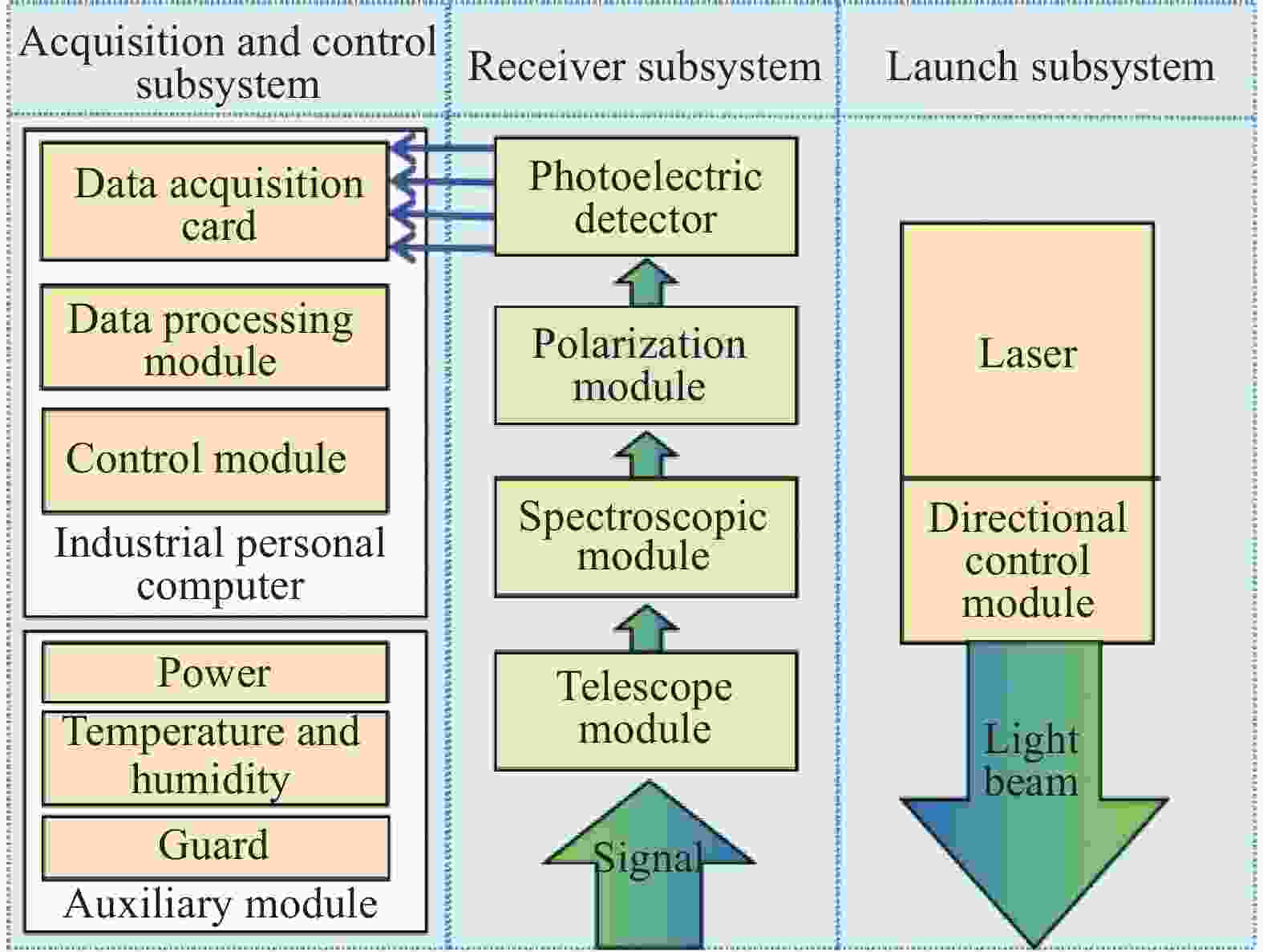
图  1  海洋激光雷达系统设计方案

Figure 1.  Oceanic lidar system design scheme

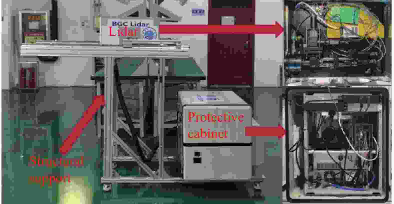
图  2  系统实物

Figure 2.  System object

发射子系统主要由激光器和反射镜组成。激光器产生486 nm和532 nm线偏振光，在激光出射口处安装两个反射镜，用于调整光束的出射方向，确保其与接收子系统的光轴平行。发射子系统的仪器性能需根据探测目标需求和工作方式进行选择，同时考虑实际的采购渠道和成本^[9]。发射子系统仪器及其性能参数如表1所示。

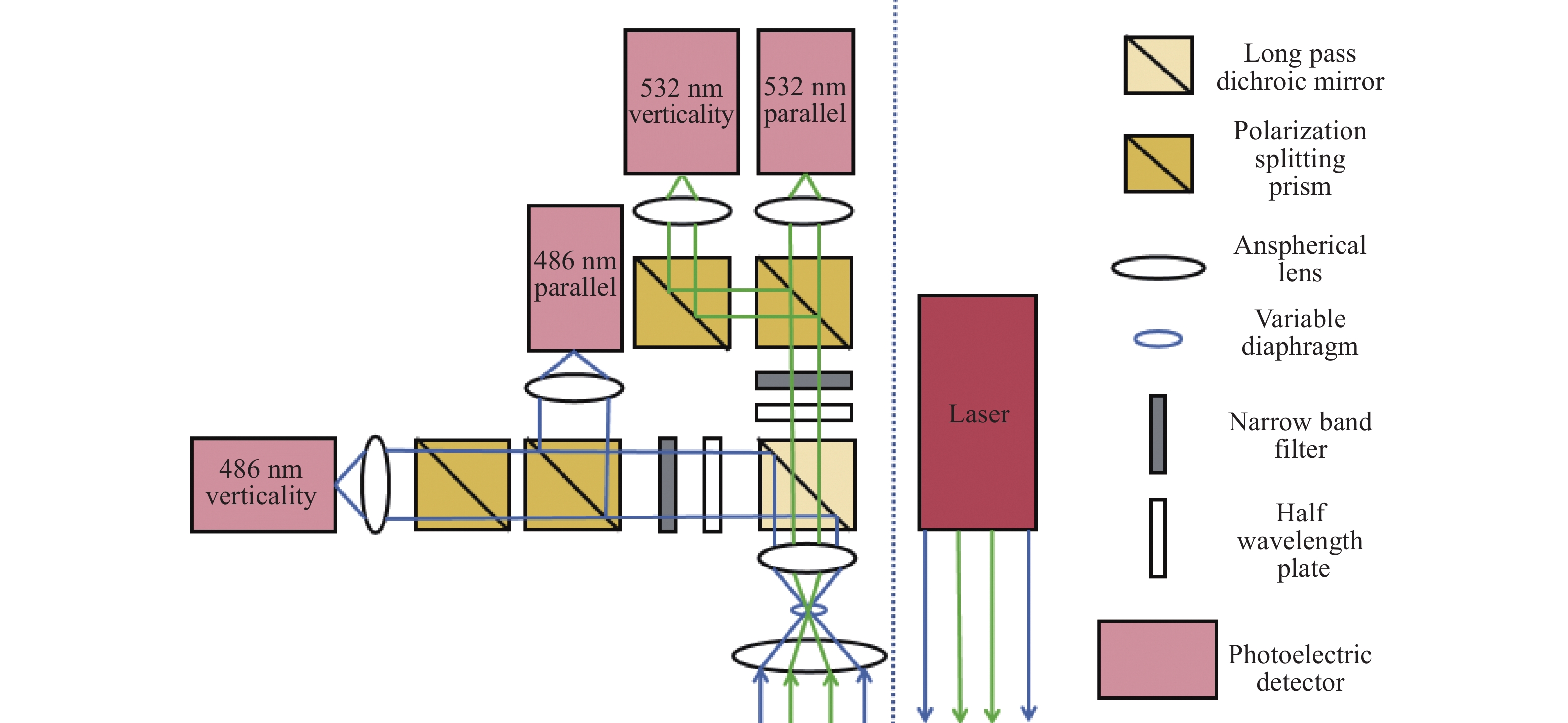
接收子系统包括望远镜、可变光阑、分光模块、偏振模块、光电倍增管等。为避免海洋表面过强的“镜面反射”信号导致光电探测器饱和，发射和接收子系统在结构上采用旁轴设计，在收发光轴平行且忽略水体多次散射和信号展宽的前提下，根据收发子系统的几何位置关系和接收视场大小，可计算出视场重叠所对应的最近探测距离^[6]。发射和接收子系统的结构设计如图3所示。

图  3  发射和接收子系统结构设计

Figure 3.  Physical design of launch and receiver subsystem

激光器发射的蓝绿光与目标相互作用后，回波光信号由接收子系统的望远镜接收并准直，其中可变光阑位于望远镜焦平面，可以根据回波信号衰减情况来调整接收视场角大小，同时抑制杂散光。准直后的平行光通过长波通二向色镜完成486 nm和532 nm通道信号光分离，进入各自的探测通道。每个通道都配置有可调的半波片，可用于调整光束的偏振态。随后，光信号经过窄带滤光片，对回波信号中的背景光和杂散光进行抑制，再经过偏振分光棱镜分离出平行和垂直信号，其中平行信号是与发射激光的偏振方向相同的回波信号，垂直信号是与发射激光的偏振方向垂直的回波信号。考虑到偏振分光棱镜无法实现100%分光，在垂直通道中安装额外的偏振分光棱镜，过滤其中的平行信号。最后，在每个通道末端安装非球面镜，将光信号聚焦到光电倍增管 (Photomultiplier tube)的光电阴极，在PMT内实现光电转换及倍增放大，最终由光电阳极输出，光信号转化为可用于进一步处理和分析的电信号。光信号转为电信号的计算方法如公式（1）所示：

式中：$ P $为望远镜接收到的回波信号光功率；$ T $为光学系统透过率；$ S $为光电倍增管阴极光谱灵敏度；$ G $为光电倍增管增益系数；$ R $为采集卡阻抗；$ V $为采集卡保存的电压信号。接收子系统仪器选型需要考虑探测目标类型、回波信号的视场范围、光学系统透过率及光电探测器的灵敏度等因素，接收子系统仪器及其性能参数如表2所示。

采集及控制子系统主要包括高速数据采集卡、计算机、控制软件和数据处理软件等，各组件的优化和协调实现系统的高效运行和信号处理。系统采用4通道、16位、1 GS/s采样率的高速数据采集卡，实现信号的高速采集，在工作过程中，通过激光器调Q触发的方式实现激光发射与信号采集的同步。计算机采用性能稳定的工控机，体积小巧及丰富的总线接口等特点使其成为理想的控制和数据处理平台，将采集到的数据存储于内部固态硬盘，同时安装调控软件。其中控制软件负责调控硬件设备参数，包括激光输出功率、高速数据采集卡采集参数等，使激光雷达可以远程控制和高效运行。数据处理软件用于对激光雷达回波数据进行预处理及水体光学特性参数的反演，有助于实时观察信号状况。采集及控制子系统的优化和协调使系统能够应对不同的水体目标需求并提供准确的数据，仪器及其性能参数如表3所示。

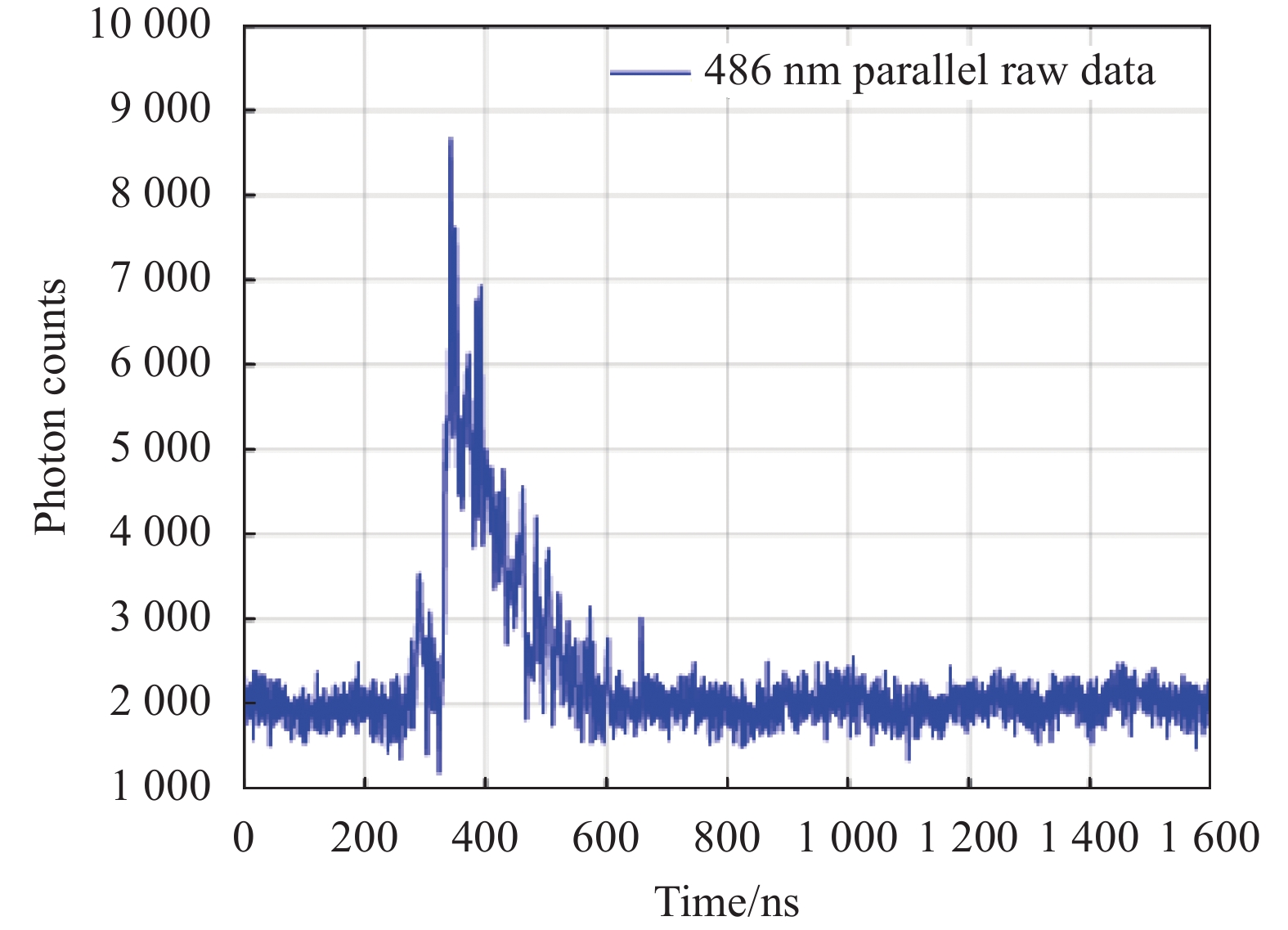
在激光雷达工作过程中，受系统硬件干扰，数据集中存在误触发信号，此外，回波信号中除了目标信号外还包括激光器Q开关干扰噪声、暗电流噪声、PMT后脉冲噪声以及环境噪声等多种背景噪声。为了获取有效的水体目标信号，需要对数据进行预处理。以486 nm平行通道数据为例介绍系统回波数据及预处理方法，如图4所示。

根据海面反射特性，回波信号的峰值强度和位置对应于海洋表面的信号强度和位置，信号中的振荡现象为激光器Q开关干扰导致。由于单脉冲信号具有偶然性，后续将采用1 min的平均信号来评估数据处理前后的回波信号质量。

图  4  486 nm平行通道单脉冲信号

Figure 4.  Monopulse signal of 486 nm parallel channel

质量控制包含两部分工作：1）通过设置峰值强度阈值过滤误触发信号；2）通过设置峰值位置阈值过滤水面以上随机目标的干扰信号，其中阈值大小基于数据集的峰值强度和位置分布特征来确定。

1 min的信号峰值强度分布如图5（a）所示，黑色离散点为误触发信号的峰值强度，其幅值相对稳定且明显小于同步获取的激光雷达回波信号的峰值强度（蓝色离散点），因此，可设置下限强度阈值来对其过滤。蓝色离散点中过强与过弱的信号一部分来自水体内生物及物质的反射信号（应保留），另一部分来自水面以上随机目标的干扰信号，可通过设置信号峰值位置阈值的方式来过滤。激光雷达回波信号的峰值位置分布如图5（b）中的蓝色柱状图所示，峰值位置呈高斯分布趋势，其位置偏差归因于以下方面：首先，船体和海面处于动态变化，导致峰值位置的部分偏差；其次，激光器存在出光时间抖动现象，影响峰值位置的分布。峰值位置相对靠后的信号为水体中生物及物质的信号（应保留），峰值位置相对靠前的信号为海面以上随机目标的干扰信号，需要进行过滤。通过对峰值位置分布进行高斯拟合来确定峰值位置阈值，结果如图5（b）中的红色曲线所示，选择99.7%的置信区间的下限位置作为阈值，在保留有效数据的同时过滤海面以上的随机目标干扰信号。过滤后信号的峰值位置分布如图5（c）所示，可见去除了海面以上（305 ns之前）的随机目标干扰信号。对比质量控制前后的1 min平均信号，如图5（d）所示，处理后信号的峰值强度提升（由5000提升到5800），信号质量得到改善。

图  5  (a) 1 min的信号峰值强度；(b) 激光雷达回波信号的峰值位置；(c) 质量控制后激光雷达回波信号的峰值位置；(d) 质量控制前后的平均信号

Figure 5.  (a) Peak intensity of 1-minute signal; (b) Peak position of lidar echo signal; (c) Peak position of lidar echo signal after quality control; (d) Average signal before and after quality control

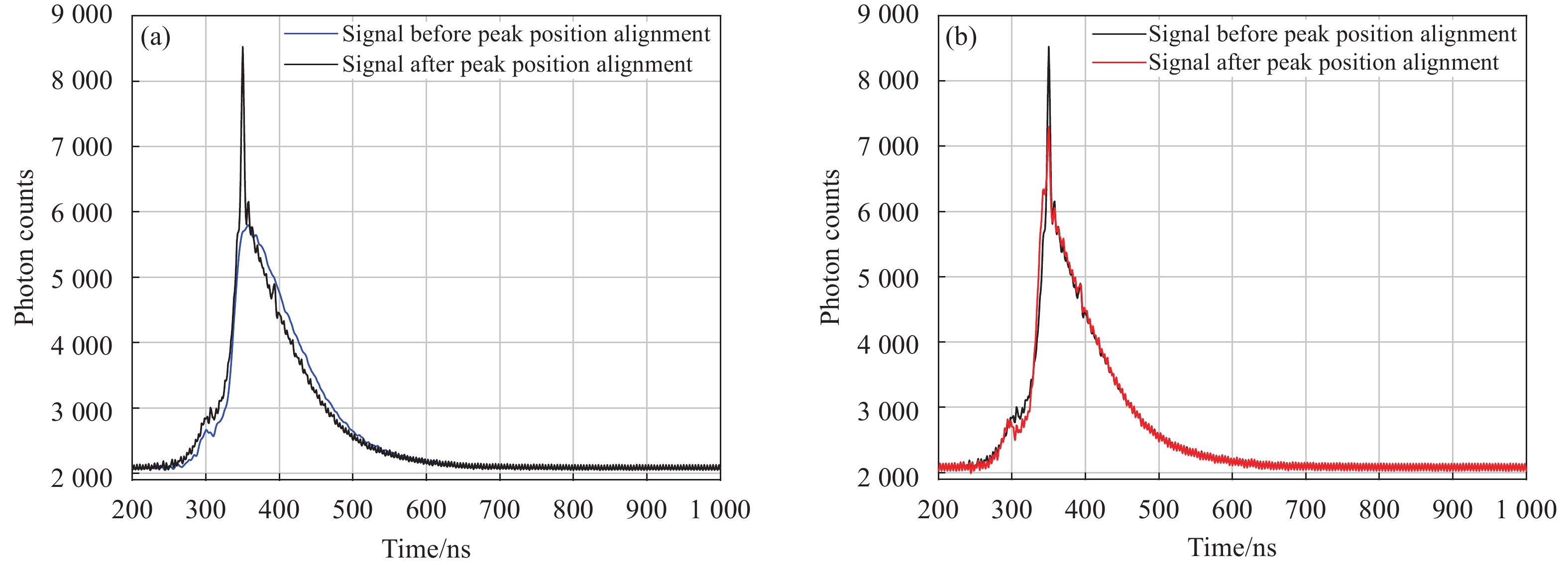
从图5（c）中观察到各脉冲的峰值位置存在偏差，因此采用峰值位置对齐的方法来减小激光器出光时间抖动以及船体晃动对位置偏差的影响。峰值对齐的步骤如下：

1）将图5（c）中峰值位置权重最大的位置视为参考位置，各脉冲峰值位置对齐到参考位置，对齐前后的平均信号如图6（a）所示，对齐后信号的峰值强度提高（由5800提高到8500），信号宽度缩小。

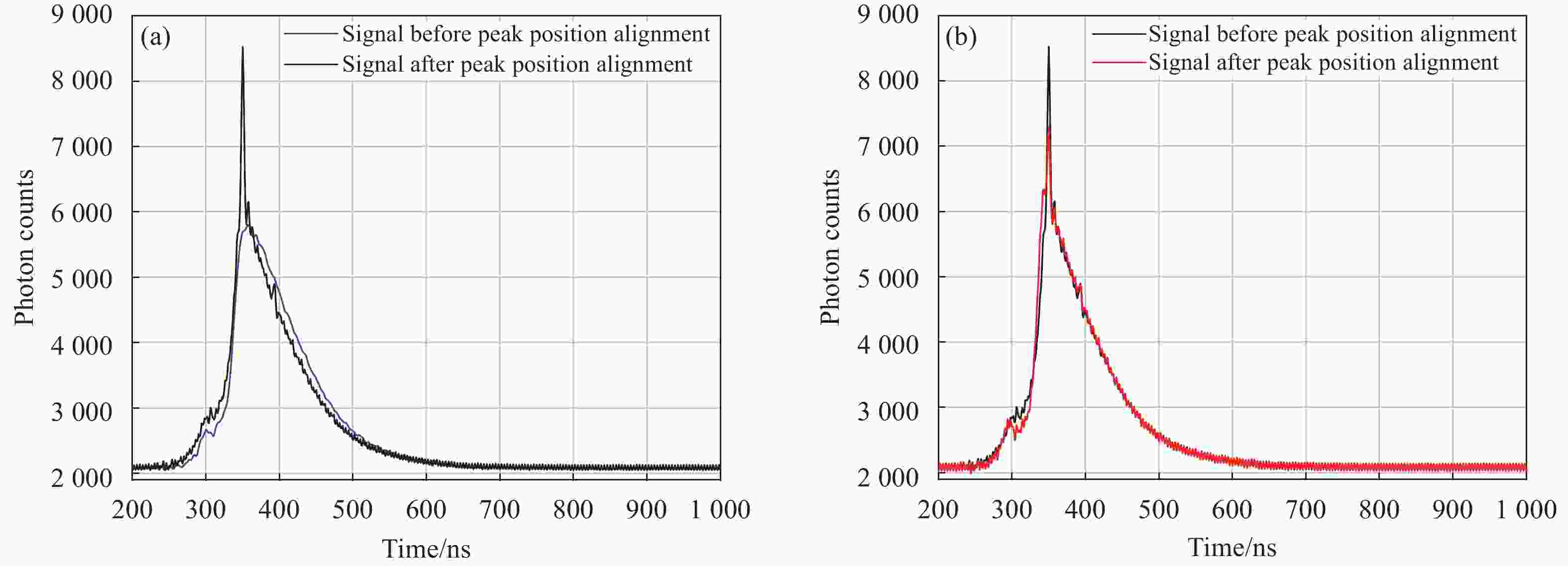
图  6  (a) 向参考位置对齐前后平均信号；(b) 依据相关性对齐前后平均信号

Figure 6.  (a) Average signals before and after alignment to the reference position; (b) Average signals before and after alignment according to correlation

2）将对齐后的平均信号（黑色曲线）作为参考信号，各脉冲信号与该参考信号进行相关性匹配，选取相关性最高的位置作为真实位置，再次进行峰值位置对齐，对齐前后的平均信号如图6（b）所示，对齐后信号宽度缩小。由图6可知，峰值位置对齐改善了信号质量。

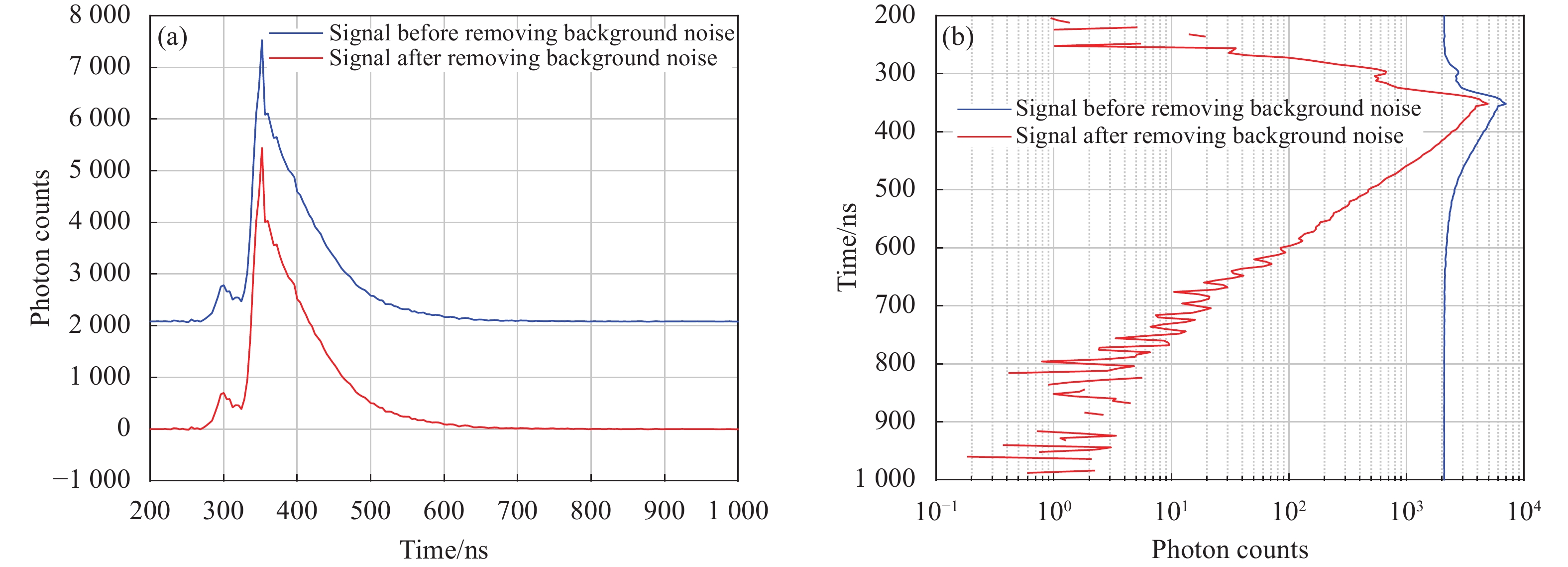
激光雷达回波信号包含目标特征信号和一系列背景噪声。为了减轻信号中激光器Q开关导致的振荡现象并保持较高的距离分辨率，对数据以4个bin大小进行叠加并取均值，随后，采用对距离足够远的回波信号进行拟合计算的方法来获取探测范围的背景噪声。对比去除背景噪声前后的平均信号，如图7（a）、（b）所示，足够远距离（900 ns之后）的信号强度由2100变为0，可见该方法有效地去除了背景噪声。

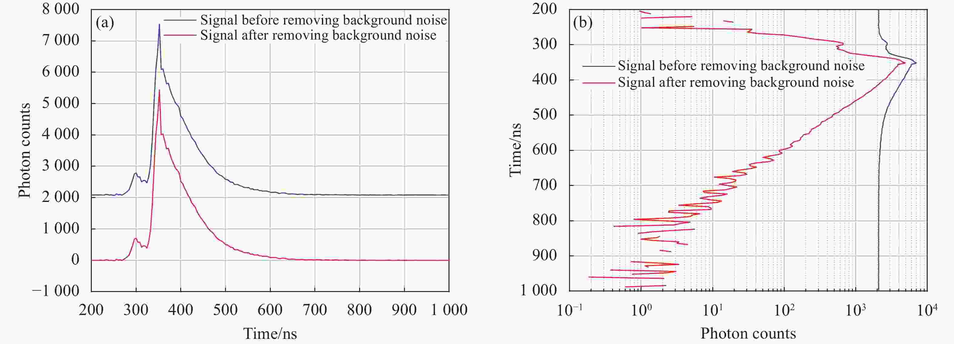
图  7  (a) 去除背景噪声前后平均信号（直角坐标系）；(b) 去除背景噪声前后平均信号（对数坐标系）

Figure 7.  (a) Average signals before and after removing background noise (rectangular coordinate system); (b) Average signals before and after removing background noise (logarithmic coordinate system)

系统采用PMT作为光电探测器，在工作过程中，PMT会产生后脉冲信号，影响对更深层微弱信号的精确测量，此外，回波信号的动态范围较大，这使得难以将目标的后向散射信号与PMT后脉冲信号分开。海洋激光雷达探测器接收到的水体后向散射信号可以视作是真实水体后向散射信号与探测器响应函数矩阵的卷积结果^[16]，可以表示为：

式中：$ {S}_{m}\left(z\right) $为探测器接收的水体后向散射信号；$ S\left(z\right) $为真实的水体后向散射信号；$ F\left(z\right) $为探测器响应函数，可通过实验室硬靶目标探测实验获取。文中采用退卷积^[16]的方法得到真实的水体回波信号，可以表示为：

为了分析平均信号在退卷积前后的变化，对退卷积后的数据以4个bin大小进行了3次平滑处理。图8（a）、（b）分别展示了直角坐标系和对数坐标系下的处理结果，退卷积后最大探测深度增加，降低了PMT后脉冲信号对数据的影响，从而优化了数据处理的效果。

图  8  (a) 退卷积前后平均信号（直角坐标系）；(b) 去退卷积前后平均信号（对数坐标系）

Figure 8.  (a) Average signals before and after deconvolution (rectangular coordinate system); (b) Average signals before and after deconvolution (logarithmic coordinate system)

为了验证系统的稳定性和可靠性，于2023年4月14日在距离大陆330 km的海域进行了定点观测实验，获取了夜间4 h （18:00-22:00）连续观测的486 nm和532 nm通道剖面数据，海况等级3级。根据MODIS卫星在该海域的数据结果显示，该海域漫衰减系数$ {K}_{d} $（490）随着离岸距离的增加数值逐渐降低，范围在 10^–2~10 m^–1 ，受陆源物质影响较小，属于干净的海洋区域。在海试期间，激光发射端口距离海面的垂直高度约为9 m，为了获取深层水体信号，系统采用宽视场（30 mrad）进行探测。在忽略激光展宽、水体折射和多次散射等因素的前提下，考虑到激光在站点观测时以30°入射水面，经过角度校正后，视场在垂直方向上的重叠位置约为7 m。为确保系统能够安全、稳定地运行，考虑太阳耀斑的强反射信号，在白天中午时分对系统的各个仪器参数进行了标定，在各通道安装衰减片，其OD值分别为1@532 nm 平行通道、1@532 nm 垂直通道、2@486 nm 平行通道、2@486 nm 垂直通道。采集时，激光的脉冲重复频率为100 Hz，采集卡的采样频率为1 GHz，为减少电脑主机的负载，确保数据的高速采集和存储，将每分钟采集的6000个脉冲信号存储为一个文件。

考虑到水体对光束的折射影响，需要对探测距离进行角度校正，从而获取垂直深度信息。系统的有效探测深度通过信噪比阈值为1来确定^[5]，在信噪比小于1的深度范围内，激光能量已衰减到一定程度，此时背景噪声过强，无法提取可靠的信号。信噪比^[9]计算方法如公式（4）所示：

式中：${N}_{{\rm{s}}}$为激光雷达接收到的目标有效信号；${N}_{{\boldsymbol{b}}}$为背景噪声。

1 min平均信号的剖面分布如图9（a）所示，可见随着深度增加，信号强度呈指数衰减趋势，与激光在水体传输中受到的水体组分吸收和散射作用有关。平行通道为激光发射信号的接收通道，信号强度较高，而垂直通道信号来自水体目标的退偏信号，强度较低，因此平行通道具有更强的探测能力。观察平行通道可以发现，486 nm比532 nm衰减速度更慢，表明486 nm具有更好的探测能力。1 min平均信号的信噪比剖面分布如图9（b）所示，可见486 nm和532 nm平行通道的有效探测深度约为30 m，而486 nm垂直通道约为27 m，532 nm垂直通道约为18 m。观察平行通道信号，在30 m深度时，486 nm的信号动态范围约为2个数量级，而532 nm约为3个数量级。

图  9  (a) 1 min平均信号剖面；(b) 1 min平均信号信噪比剖面

Figure 9.  (a) Profile of 1-minute average signal; (b) SNR profile of 1-minute average signal

4 h连续观测的蓝绿通道回波信号如图10（a）、（b）所示，总体来看，在相同的数量级范围内，486 nm相比于532 nm能获取更大范围的水体信号，具有更好的探测能力。

图  10  (a) 4 h 532 nm平行通道信号剖面；(b) 4 h 486 nm平行通道信号剖面

Figure 10.  (a) Signal profile of 4-hour 532 nm parallel channel; (b) Signal profile of 4-hour 486 nm parallel channel

激光穿过介质的过程中会产生延时、频移、吸收、散射等现象，通过分析回波信号的光谱、波形、强度、频移等特征，能够获得探测深度的目标光学特性信息^[4]。描述海洋激光雷达回波信号的一般弹性激光雷达方程^[4]如公式（5）所示：

式中：$ S\left(z\right) $为海洋激光雷达回波信号；$ z $为散射物体到海洋表面的垂直深度；H为激光雷达到水面的高度；$ C $为系统常数；$ \beta (\pi ,z) $为180°体积散射系数；${K}_{{\rm{lidar}}}$为水深$ z $处的激光雷达衰减系数。考虑公式（5）同时具有两个光学特性参数变量，采用斜率法^[17]来计算激光雷达衰减系数，如公式（6）所示：

为了分析激光雷达衰减系数的分布规律，对数据以8个bin的窗口进行平滑处理，激光雷达衰减系数剖面分布如图11（a）、（b）所示。受到海洋上层水体过饱和信号干扰及水体多次散射导致的视场未重叠等问题的影响^[18]，上层水体的激光雷达衰减系数不可用，因此，选择水面6 m以下的有效探测深度内的4 h平均激光雷达衰减系数进行分析，如图12所示。

图  11  (a) 4 h 532 nm平行通道激光雷达衰减系数剖面；(b) 4 h 486 nm平行通道激光雷达衰减系数剖面

Figure 11.  (a) Lidar attenuation coefficient profile of 4-hour 532 nm parallel channel; (b) Lidar attenuation coefficient profile of 4-hour 486 nm parallel channel

图  12  激光雷达衰减系数

Figure 12.  Attenuation coefficient of lidar

在有效探测深度内，可见486 nm和532 nm的激光雷达衰减系数均随着深度的增加逐渐增大，该衰减趋势与水体各组分的吸收和散射作用有关，数据结果与文献[18]中的水体叶绿素浓度剖面和激光雷达衰减系数剖面的分布趋势相似。在相同探测深度内，即使绿光发射能量更高，约为蓝光的1.5倍，与532 nm相比，486 nm通道的激光雷达衰减系数较小，表明在清洁大洋水域，486 nm波长具备更好的探测能力，能够获取更深层的水体信息。

船载蓝绿光海洋激光雷达系统在清洁大洋水域获取了蓝绿波段的水体后向散射回波信号及激光雷达衰减系数的剖面信息。数据结果表明：在开阔水域中，相较于532 nm，486 nm的激光雷达衰减系数更小，具有更出色的探测性能；激光雷达系统在486 nm和532 nm波长分别能够在2个和3个数量级的动态范围内获得有效探测深度约30 m的光学特性参数剖面。数据结果验证了系统的可靠性，检验了蓝绿波长探测通道的工作性能，为海洋激光雷达在海洋探测领域的应用潜力提供了有力支持。未来将进一步优化系统的软硬件设计，探究海洋激光雷达系统误差来源，提高数据的精确性。同时，将开展更多水域的探测实验，反演多种水体光学特性参数，并与机载数据和原位仪器实测数据进行对比验证，以进一步验证系统的可靠性和适用性。

致 谢 ：感谢崂山实验室海洋高端仪器设备研发平台提供支持。