


-
发射率是表征物质表面辐射能力的重要物理量,是重要的热物理参数,在许多领域中都有着极为重要的应用[1]。在航空航天领域,飞行器在气动加热中,机身会与空气之间摩擦产生过高温度导致机身过热,对飞行器热防护系统的散热性能提出了很高的要求,而飞行器散热主要是辐射散热,表征材料热辐射能力大小的发射率便成为了决定飞行器蒙皮散热效率的重要评判指标[2]。在国防军事领域中,发射率是飞行器红外隐身的关键技术之一[3],战机利用低发射率减小热辐射性能的涂层来隐藏目标,躲避红外追踪,从而使其很难被探测器监视到,以实现隐身效果[4-5]。
综上所述,发射率在许多应用领域中有着极其重要的地位,同时随着国防科技、太阳能研究、辐射测温、材料科学的发展,众多应用领域对发射率的测量技术有了更高的需求。自1970年起,日本东洋大学的 Tohru Iuchi开始了对发射率测量装置和不同材料发射率特性的研究[6]得到了发射率与材料的种类、温度以及波长有关;日本东北大学先进材料多学科研究所于2020年研制了一套发射率测量装置,用于研究液态Ni-Al合金法向光谱发射率的成分依赖特性[7-9];丁经纬[10]等制作了几种不同的高发射率黑体涂层,并基于中国计量科学研究院的发射率测量装置得到了高发射率黑体涂层的辐射特性;北航联合先进航空发动机协同创新中心研制了一套光谱范围可达1~15 μm,温度范围为400~1200 K的发射率测量装置,开展了大量对高温镍基合金红外法向光谱特性的研究[11];河南师范大学刘玉芳团队研制了一套在5~20 μm 波长范围内测量不同温度下固体材料的光谱发射率测量装置[12-13];北京理工大学的袁良等[14]基于发射率定义建立了材料法向光谱发射率测量模型,研制了一套0.7~12 μm的材料法向光谱发射率测量装置。
发射率并非物体的本征属性,而是一个很难准确测量的物理量,与温度、波长、角度等有关,其测量较为复杂,目前发射率测量方法大都只是对某一单一物质进行接触式测量,难以获得复杂目标的发射率三维分布。随着近年来红外激光雷达成像技术的发展,对于红外激光雷达的应用也有了新的发展。激光雷达(Light Detection and Ranging,LiDAR)是一种通过发射特定波长的激光以获取距离、反射率等相关信息的主动式探测技术[15],除了获取扫描目标高密度、高精度的三维空间信息外,还能通过光电接收系统记录目标对发射激光的后向散射回波强度。回波强度作为点云的最重要特征之一,表征目标对激光的反射光谱特性,是反映目标辐射特性的重要物理量[16]。利用回波强度的反射光谱特性计算出目标表面的反射率,通过反射法进而推导出目标表面的发射率。
综上所述,针对目前发射率测量方法只是对某一单一物质进行接触式测量,难以获得复杂目标的发射率三维分布,结合M8线阵激光雷达的高精度、高分辨率,抗干扰能力强等优势,基于M8激光雷达回波提出一种非接触式发射率三维分布测量方法。测量方法原理示意图如图1所示。通过M8激光雷达对95%标准漫反射板进行线阵扫描,叠加多帧单线点云,得到具有反射光谱特性的雷达强度三维点云像;运用分段多项式模型拟合距离-强度及入射角-强度之间的关系,基于分段多项式模型校正距离和入射角度影响下的回波强度,使标准漫反射板强度整体趋于一致,提升回波强度数据有效,使不同距离与入射角情况下所测回波强度能够真实地反映目标的反射光谱特性,验证强度校正模型的有效性;最后采用分段多项式校正模型对带有反射率真值贴片的缩比卫星模型雷达强度三维点云像进行强度校正,利用校正后的回波强度的反射光谱特性计算出目标表面的反射率,运用反射法进一步推导其发射率,得到缩比卫星模型发射率的三维分布,实现非接触式目标发射率三维分布测量,可同步识别目标表面材料属性,获得目标三维几何特征,能在现代战争中大大提升对军事目标的认知能力。

图 1 测量方法原理示意图
Figure 1. Schematic diagram of the principle of measurement method
-
激光雷达通过向目标发射一束窄而锥形的光束,记录扫描物体反向散射返回的激光脉冲信号,整个扫描过程遵循雷达距离方程。对于扩展目标,雷达距离方程可简化为:
$$ {P_r} = \frac{{{P_t}{D_r}^2}}{{4\pi {R^4}{\beta _t}^2}}\sigma {\eta _{{\rm{sys}}}}{\eta _{{\rm{atm}}}} $$ (1) 式中:${P_r}$为接收激光功率;${P_t}$为发射激光功率;${D_r}$为接收机孔径直径;$R$为雷达扫描中心到扫描目标点距离;${\beta _t}$为发射器波束宽度(${\beta _t}$很小);${\eta _{{\rm{sys}}}}$为系统透射因子;${\eta _{{\rm{atm}}}}$为大气透射因子;$\sigma $为后向散射截面。$\sigma $可表示为:
$$ \sigma = \frac{{4\pi }}{\varOmega }\rho {A_s}\cos \theta $$ (2) 式中:$\varOmega$为实心角;$\rho $为激光波长处的目标反射率;${A_s} = \dfrac{{\pi {R^2}\sin \beta _t^2}}{4} \approx \dfrac{{\pi {R^2}\beta _t^2}}{4}$为目标有效接收区域。
后向散射截面的方向和回波强度都受到目标反射类型(如镜面反射或漫反射)的影响。如果目标为朗伯体,则会发生漫反射[17]。辐射均匀地散射到一个半球,而不是像镜面反射那样只在一个方向上,如图2所示,即公式(2)中$\varOmega = \pi$。根据朗伯体余弦定律,后向散射截面与入射角的余弦$\theta $成正比。公式(1)可简化为:
$$ {P_r} = \frac{{{P_t}D_r^2\rho \cos \theta }}{{4{R^2}}}{\eta _{{\rm{sys}}}}{\eta _{{\rm{atm}}}} $$ (3) 式中:${P_t}$、${D_r}$、${\eta _{{\rm{sys}}}}$和${\eta _{{\rm{atm}}}}$均可被认为是常数。将所有常数合并后,将公式(3)进一步简化为:
$$ {P_r} = K \cdot \rho \cdot \cos \theta \cdot {R^{ - 2}} $$ (4) 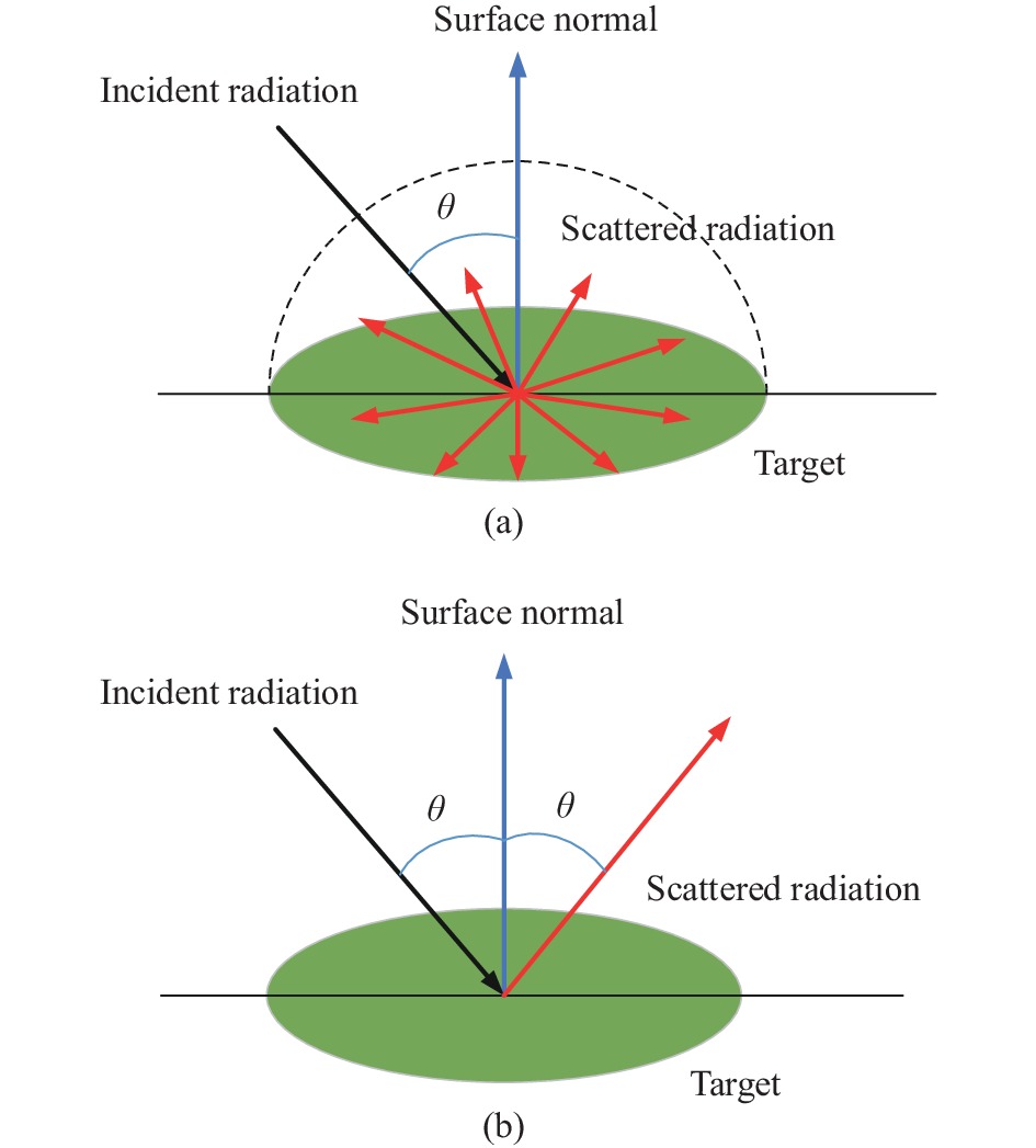
图 2 漫反射(a) 及镜面反射(b)
Figure 2. Diffuse reflection (a) and specular reflection (b)
激光雷达所记录的回波强度I通常被假定为接收到的回波的信号振幅(峰值功率),即强度值与在特定时间间隔内撞击探测器的光子数量成正比[18]。因此:
$$ I\infty {P_r}\infty \rho \cdot \cos \theta \cdot {R^{ - 2}} $$ (5) 由公式(5)可知,回波强度值I与入射角余弦值成正相关,与距离的平方成负相关。当距离恒定时,目标与激光雷达扫描时所处相对位置的不同会使单次扫描时入射角存在差异,导致回波强度值在不同的入射角时会得到不同的值。
然而,大多数自然曲面都不是理想的朗伯体曲面,回波脉冲可能会被扭曲。距离和入射角对原始强度的影响在理论上是相互独立的,可以分别进行校正,如公式(6)所示:
$$ I(\lambda ,R,\theta ) = {f_\lambda }(\lambda ){f_r}(R){f_\theta }(\cos \theta ) $$ (6) 式中:$I(\lambda ,R,\theta )$为原始强度;${f_\lambda }(\lambda )$、${f_r}(R)$、${f_\theta }(\cos \theta )$分别表示目标反射率、距离和入射角独立影响的函数。为消除距离和入射角对强度的影响,对于具有相同反射率的朗伯体,应将任意距离和入射角处的$I(\lambda ,R,\theta )$转化为参考距离${R_0}$和参考入射角${\theta _0}$处的校正强度${I_c}$:
$$ \begin{gathered} {I_{{c}}} = {f_\lambda }(\lambda ){f_r}\left( {{R_0}} \right){f_\theta }\left( {\cos {\theta _0}} \right) = \frac{{{f_r}\left( {{R_0}} \right){f_\theta }\left( {\cos {\theta _0}} \right)}}{{{f_r}(R){f_\theta }(\cos \theta )}} \cdot I(\lambda ,R,\theta ) \\ \end{gathered} $$ (7) -
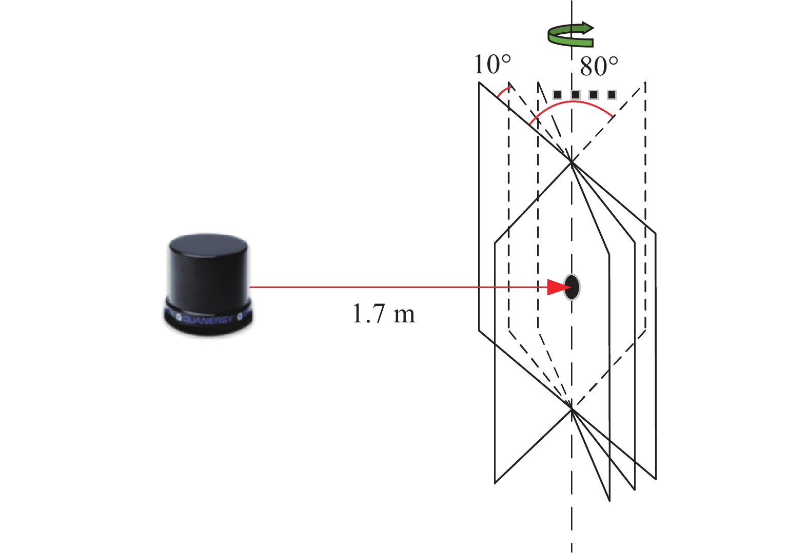
采用8线M8线阵激光雷达,波长为905 nm,帧率1~20 Hz,扫描选取帧率1 Hz,在45°视场,该激光雷达采集的点数为4800个/s。
M8激光雷达静止不动时,通过雷达自身旋转中心,只能获取前方一个固定视场的线状点云信息,如图3所示。文中通过单轴自由转台搭载M8激光雷达,通过转台带动X轴,实现对目标的线阵扫描,如图4所示。

图 3 激光雷达固定视场线状点云
Figure 3. Linear array LiDAR point cloud in fixed field of view

图 4 雷达扫描成像示意图
Figure 4. Schematic diagram of LiDAR scanning imaging
-
单轴自由转台搭载雷达进行扫描时,8条扫描线会先后依次扫描目标,即每条单线均会储存相同的目标点云数据,同时,进行多线的数据叠加会造成数据冗余,极大地提升后续点云数据的处理难度,因此选取8线中的居中单线数据进行多帧单线叠加。
发射与接收传感器在竖直方向上按照单向旋转周期性运动,在水平方向上按照步进的方式运动,则在T时刻雷达传感器发射的激光角度可以表示为:
$$ \begin{array}{*{20}{l}} {{\theta _d} = d + T \cdot \Delta \alpha } \\ {{\theta _h} = h + T \cdot \Delta \beta } \end{array} $$ (8) 式中:${\theta _d}$为T时刻激光所在的水平位移角度;d为光线最大偏移角度在水平方向上的初始位移分量;$\Delta \alpha $为单位时间内水平方向变化位移;${\theta _h}$为T时刻激光所在的竖直角度位移;h为光线最大偏移角度在竖直方向上的初始位移分量;$\Delta \beta $为单位时间内竖直方向的位移变化角度。
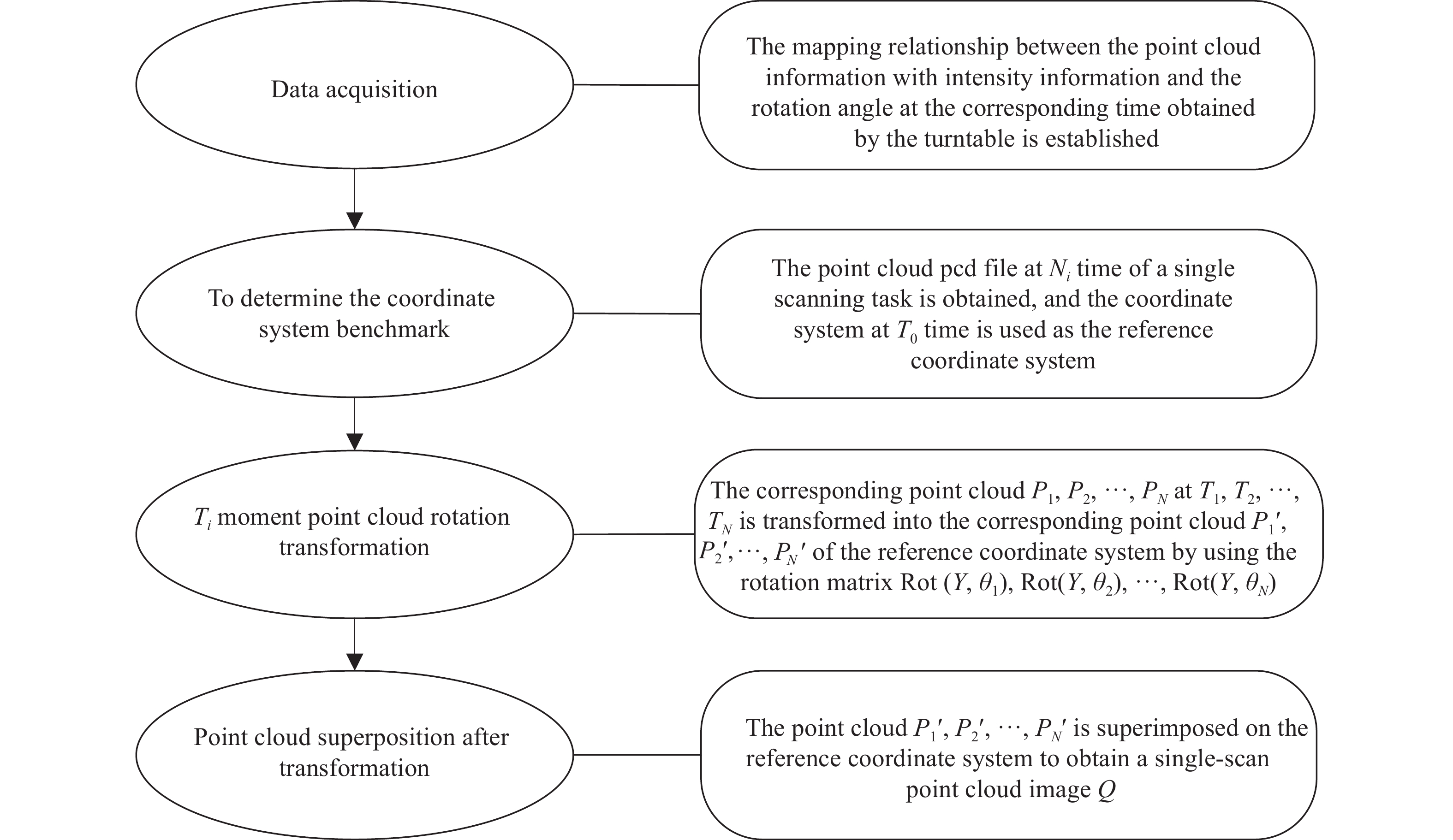
点云数据处理算法实现过程具体如图5所示。转台旋转中心与雷达传感器的Y轴重合。单次扫描周期内不同时刻下扫描时,转台搭载激光传感器的位置不同,扫描得到的点云数据坐标系不统一,需要统一在一个基准坐标系内处理数据。以第一帧点云所对应的雷达坐标系为该次扫描结果点云的坐标系,将该次扫描的点云按照旋转角度旋转到对应的基准位置。
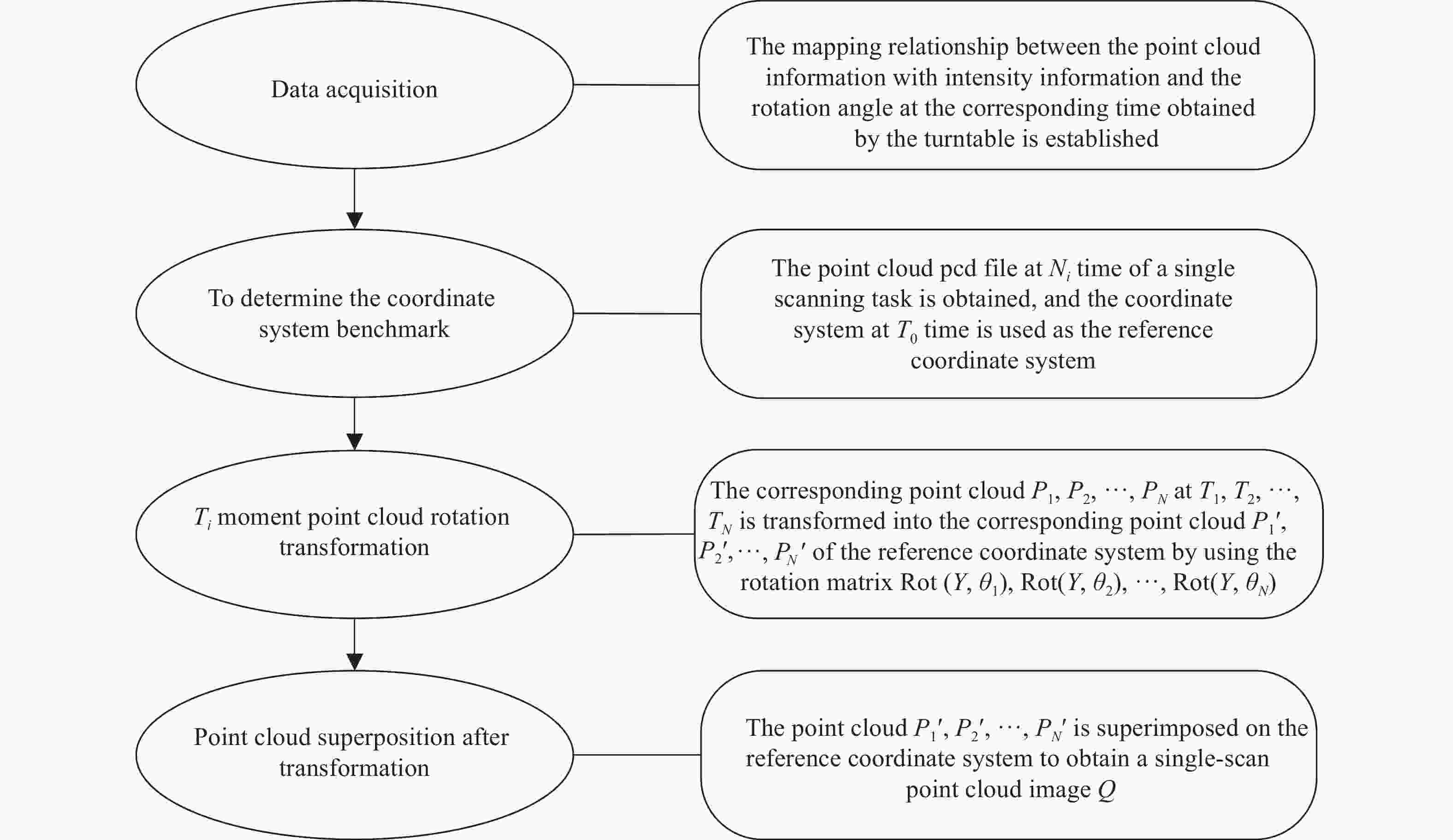
图 5 点云数据处理算法流程图
Figure 5. Flow chart of point cloud data processing algorithm
-
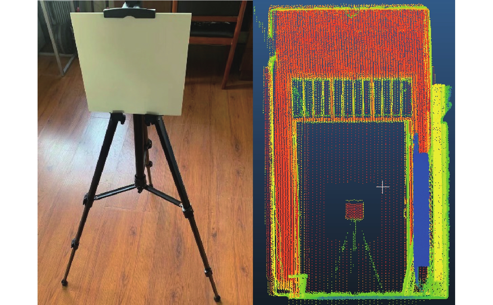
参考目标为95%反射率标准漫反射板,对应波长为905 nm,尺寸为20 cm×20 cm,如图6所示。漫反射板由高度漫反射的材料组成。当波长为905 nm的激光束照射时,漫反射板可视为标准朗伯体。

图 6 95%反射率标准漫反射板
Figure 6. 95% reflectivity standard diffuse reflector
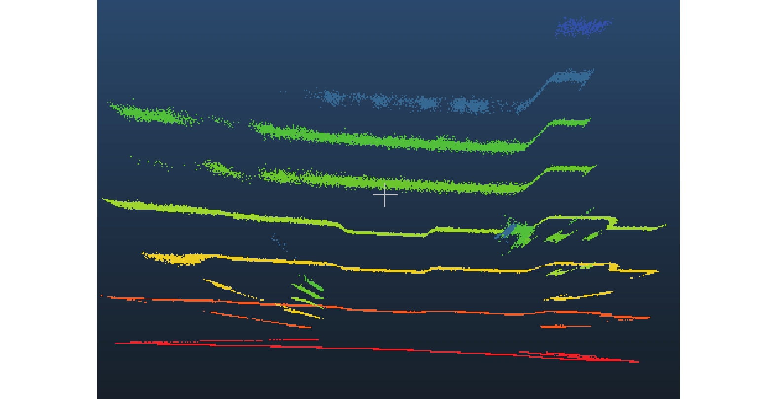
图7所示为带有背景的目标样板点云回波强度三维点云像,通过对目标点云进行X、Y、Z阈值划分,即目标样板主体部分在x、y、z维度方向上的最大值与最小值坐标值确定三个维度的阈值范围xmin,xmax,ymin,ymax,zmin,zmax,实现对标准漫反射板提取,如图8所示。

图 7 带有背景的目标样板回波强度像
Figure 7. Target template echo intensity image with background

图 8 标准漫反射板回波强度点云像
Figure 8. Standard diffuser echo intensity point cloud image
-
原始回波强度数据会受到目标反射率的影响,扫描距离、入射角和大气衰减效应等因素使得目标反射率产生偏差,需校正这些系统变量,消除其他因素对强度值的影响,使得强度值能直接反映目标的反射光谱特性。
强度信息受制于硬件(光源、探测器等),对特定仪器来说是唯一的,很难进行绝对校正,必须结合硬件特点和探测物体本身的特点来校正,且不同厂商的激光雷达对回波强度的单位和数值尺度的表述并不一致,即便是来自同一厂商的不同激光雷达,在扫描同一目标时,回波强度值也会存在差异。故文中校正方法仅适用于905 nm M8线阵激光雷达扫描获取的目标点云的强度数据。
-
雷达扫描过程遵循雷达距离方程,回波强度会随着距离的改变而改变,需对校正方程里的参考距离进行标定,使参考距离下的强度值能直接反映目标材料的反射特征,采用95%、50%、2%标准漫反射板进行联合标定,三者均为标准朗伯体,理论上,在参考距离下三者的强度应成对应比例关系,标定试验示意如图9所示。

图 9 参考距离标定试验
Figure 9. Reference distance calibration test
为了验证标定的有效性,在相同条件下分别对蓝色亚光板(22%)、绿色亚光板(18%)、白色亚光板(62%)、黑色亚光板(4%)进行强度数据采集,括号里的数值为四块亚光板在恒温条件下采用光谱仪测得的905 nm波段下的反射率,通过与标准板的比对,如表1所示,1.7 m的条件下,七个试验样板所测的强度值能够接近或满足反射率之间的对应关系,即1.7 m下雷达所测的强度值能够反映目标真实的反射特征。将1.7 m作为参考距离,对回波强度进行校正。
表 1 不同距离下标定样板的强度值
Table 1. Strength value of the calibration template at different distances
Group 95% 50% 2% Blue
(22%)Green
(18%)White
(62%)Black
(4%)0.5 m 8 8 0 0 0 8 0 1.0 m 38 23 0 0 0 30 0 1.5 m 68 45 0 15 8 23 0 1.7 m 83 45 0 23 23 45 0 2.0 m 91 68 0 61 61 77 15 2.4 m 121 98 0 98 76 122 76 3.1 m 159 136 0 121 128 151 113 -
选取标准反射板作为扫描对象,固定入射角及其他影响因素,设置参考入射角为0°,以0.7 m为间隔改变目标的激光测距值,在相同的视场角下采用激光雷达对标准漫反射板进行线阵扫描,如图10和图11所示。可获得标准漫反射板带有回波强度值的点云信息,得到激光雷达测距值与回波强度的关系,如图12所示。

图 10 参考入射角0°时1~15 m强度测量示意图
Figure 10. Strength measurements at different positions of 1-15 m at a reference incident angle of 0°

图 11 参考入射角0°时1~15 m强度测量场景图
Figure 11. Referring to the real scene of 1-15 m intensity measurement at the incident angle of 0°

图 12 参考入射角0°时雷达测距值与回波强度的关系
Figure 12. The relationship between LiDAR ranging value and echo intensity when the reference incident angle is 0°
标准漫反射板满足恒定的反射率,以恒定的入射角对进行不同距离R进行扫描,则距离校正后的强度${I_{rc}}$为:
$$ \begin{gathered} {I_{rc}} = \frac{{{f_r}\left( {{R_0}} \right){f_\theta }\left( {\cos {\theta _0}} \right)}}{{{f_r}(R){f_\theta }\left( {\cos {\theta _0}} \right)}} \cdot I(\lambda ,R,\theta ) {\text{ }} = \frac{{{f_r}\left( {{R_0}} \right)}}{{{f_r}(R)}} \cdot I(\lambda ,R,\theta ) \\ \end{gathered} $$ (9) 式中:Rmin≤R≤Rmax(Rmin和Rmax分别为距离测量范围的最小值和最大值)。根据Weierstrass定理[19],闭合区间的连续函数可以用多项式级数一致逼近。
根据定义,${f_r}(R)$描述了距离强度数据中距离R与$I(\lambda ,R,\theta )$之间的关系。通过距离多项式拟合得到反射率$\lambda $和参考入射角${\theta _0}$下的强度值$I(\lambda ,R,{\theta _0})$。Tan和Cheng[20]表明,由于雷达光学系统的短距离效应,当距离较近时,强度随着距离的增加而增加,当距离较远时,强度随着距离的增加而降低。根据距离R变量,可采用分段多项式建立校正模型,如公式(10)所示:
$$ {f}_{r}(R)=I\left(\lambda ,R,{\theta }_{0}\right)=\left\{\begin{array}{ll}{\displaystyle \sum _{k=0}^{K}\left({a}_{k}{R}^{k}\right)}, & R < {R}_{s} \\ {\displaystyle \sum _{m=0}^{M}\left[{b}_{m}{\left({1}/{R}\right)}^{m}\right]}, & R\geqslant{R}_{s} \end{array}\right. $$ (10) 式中:${a_k}$和${b_m}$为距离多项式的系数;k和m为距离多项式的阶数;Rs为距离分界点。
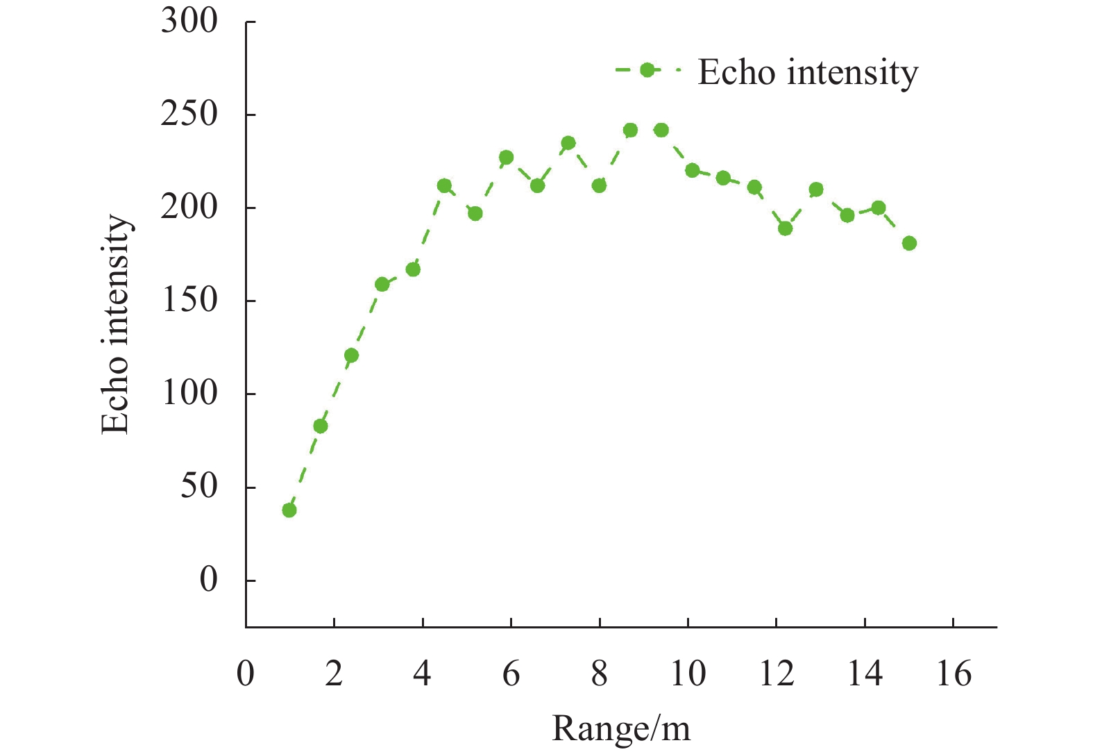
从图12中可以看出,随着测量距离的增加,回波总体呈现强度先增加后减小趋势,在R=8.7 m时回波强度达到最大值,因此选择8.7 m这个极值点作为分段函数的临界点Rs,即Rs=8.7 m。
结合公式(9)可得:
$$ {I_{rc}} = \frac{{{f_r}\left( {{R_0}} \right)}}{{{f_r}(R)}} \cdot I(\lambda ,R,\theta ) = \left\{ {\begin{array}{*{20}{l}} {\frac{{I(\lambda ,R,\theta )\displaystyle\sum\limits_{k = 0}^K {{a_k}} {R_0}^k}}{{\displaystyle\sum\limits_{k = 0}^K {{a_k}} {R^k}}},}&{R \leqslant {R_s}} \\ {\frac{{I(\lambda ,R,\theta )\displaystyle\sum\limits_{m = 0}^M {{b_m}} {{\left( {1/{R_0}} \right)}^m}}}{{\displaystyle\sum\limits_{m = 0}^M {{b_m}} {{(1/R)}^m}}},}&{R > {R_s}} \end{array}} \right. $$ (11) -
通过固定激光测距值及其他影响因素改变标准漫反射板与激光雷达的相对位置,使激光雷达以不同的入射角对目标进行线阵扫描,进行入射角校正试验,如图13所示,得到参考距离条件下激光入射角与回波强度的关系,如图14所示。

图 13 参考距离1.7 m时入射角0°~80°的强度测量
Figure 13. Intensity measurement at different sites of 0°-80° at areference distance of 1.7 m

图 14 参考距离为1.7 m时雷达入射角与回波强度的关系
Figure 14. The relationship between LiDAR incident angle and echo intensity when the reference distance is 1.7 m
标准漫反射板满足恒定的反射率,以不同的入射角$\theta $和恒定的距离R0扫描标准反射样板,入射角的校正强度$ {I_{\theta {\text{c}}}} $如公式(12)所示:
$$ \begin{gathered} {I_{\theta {\text{c}}}} = \frac{{{f_r}\left( {{R_0}} \right){f_\theta }\left( {\cos {\theta _0}} \right)}}{{{f_r}\left( {{R_0}} \right){f_\theta }(\cos \theta )}} \cdot I(\lambda ,R,\theta ) = \frac{{{f_\theta }\left( {\cos {\theta _0}} \right)}}{{{f_\theta }(\cos \theta )}} \cdot I(\lambda ,R,\theta ) \\ \end{gathered} $$ (12) 根据Weierstrass定理,也可通过多项式拟合得到参考反射率$ \lambda $和参考距离${R_0}$下的强度值$ I(\lambda ,{R_0},\theta ) $。用余弦多项式对$ {f_\theta }(\cos \theta ) $建立校正模型,如公式(13)所示:
$$ {f_\theta }(\cos \theta ) = I\left( {\lambda ,{R_0},\theta } \right) = \sum\limits_{n = 0}^N {{c_n}} {(\cos \theta )^n} $$ (13) 式中:${c_n}$为入射余弦多项式的系数;n为入射余弦多项式的阶数。将公式(13)代入公式(12)可得:
$$ \begin{gathered} {I_{\theta c}} = \frac{{{f_\theta }\left( {\cos {\theta _0}} \right)}}{{{f_\theta }(\cos \theta )}} \cdot I(\lambda ,R,\theta ) = \frac{{I(\lambda ,R,\theta )\displaystyle\sum\limits_{n = 0}^N {{c_n}} {{\left( {\cos {\theta _0}} \right)}^n}}}{{\displaystyle\sum\limits_{m = 0}^N {{c_n}} {{(\cos \theta )}^{\text{n}}}}} \\ \end{gathered} $$ (14) -
利用最小二乘法对${f_r}(R)$和$ {f_\theta }(\cos \theta ) $分别进行多项式拟合,选取不同的幂K、M、N,利用参与拟合的点与拟合函数的均方根误差(RMSE)作为${f_r}(R)$和$ {f_\theta }(\cos \theta ) $多项式阶数选取依据。
$$ \begin{split} {{ RMSE }}& = \sqrt {\frac{{S\left( {{a_0},{a_1}, \cdots {a_K}} \right)}}{L}} =\\& \sqrt {\frac{{\displaystyle\sum\limits_{l = 1}^L {{{\left( {I{{\left( {\lambda ,R,{\theta _0}} \right)}_l} - I{{(\lambda ,R,\theta )}_l}} \right)}^2}} }}{L}} \end{split} $$ (15) 式中:$ I\left( {\lambda ,R,{\theta _0}} \right) $为参考入射角$ \theta_{0} $下,多项式拟合函数中不同距离所对应的强度值;$ I\left( {\lambda ,R,\theta } \right) $为不同距离所对应的原始强度值;L为样本数量。
RMSE值越小,拟合误差越小,多项式阶越高(K、M、N值越大),如表2所示,但拟合阶值选择过高,将距离校正模型应用于实际场景进行强度校正时容易出现过拟合,校正效果较差;如果阶值过低,则无法有效地进行距离强度校正。为了避免过拟合,最终确定K=4、M=4、N=2。
表 2 不同阶数下多项式拟合函数均方根误差
Table 2. Root mean square error of polynomial fitting function under different orders
Order RMSE K M N 1 26.34 8.42 2.84 2 11.92 7.65 2.76 3 10.06 7.28 2.73 4 9.65 5.98 1.96 5 9.44 5.98 1.86 6 9.17 5.90 0.89 为求RMSE最小值下的各个多项式系数$ a_{k} $、$ b_{m} $、$ c_n $,将公式(10)的短距离项(Rs≤8.7 m)代入公式(15),将各多项式系数$ a_{k} $、$ b_{m} $、$ c_n $的偏导数转化为求极值问题,因此:
$$ \begin{array}{*{20}{c}} {\dfrac{{\partial S\left( {{a_0},{a_1}, \cdots {a_K}} \right)}}{{\partial {a_k}}} = } {2\displaystyle\sum\limits_{l = 1}^L {\left( {\displaystyle\sum\limits_{k = 0}^K {{a_k}} {R_l}^k - I{{(\lambda ,R,\theta )}_l}} \right)} {R^k} = 0} \end{array} $$ (16) 即:
$$ \sum\limits_{k = 0}^K {{a_k}} R_l^k = I{(\lambda ,R,\theta )_l} $$ (17) 通过公式(17)可得线性公式(18):
$$ \left[ {\begin{array}{*{20}{c}} {R_1^0}&{R_1^1}& \cdots &{R_1^k} \\ {R_2^0}&{R_2^1}& \cdots &{R_2^k} \\ \vdots & \vdots & \ddots & \vdots \\ {R_l^0}&{R_l^1}& \cdots &{R_l^k} \end{array}} \right]\left[ {\begin{array}{*{20}{c}} {{a_0}} \\ {{a_1}} \\ \vdots \\ {{a_k}} \end{array}} \right] = \left[ {\begin{array}{*{20}{c}} {I{{(\lambda ,R,\theta )}_1}} \\ {I{{(\lambda ,R,\theta )}_2}} \\ \vdots \\ {I{{(\lambda ,R,\theta )}_l}} \end{array}} \right] $$ (18) 用高斯消元法得到${a_0},{a_1},{a_2} \cdots {a_k}$,同理将公式(10)的长距离多项式(Rs>8.7 m)和公式(13)余弦多项式代入公式(15)得到${b_0},{b_1},{b_2} \cdots {b_m}$和${c_0},{c_1},{c_2} \cdots {c_n}$。即${a_0}$=−24.116,${a_1}$=61.2436,$ {a_2} $=3.6745,${a_3}$=−2.0008,$ {a_4} $=0.1314;${b_0}$=−7.993×10³,${b_1}$=3.741×10⁵,${b_2}$=−6.352×10⁶,${b_3}$=47.45×10⁶,${b_4}$=−131.186×10⁶;${c_0}$=12.5477,${c_1}$=54.826,${c_2}$=10.66,如表3所示。可得距离和入射角余弦多项式的分段多项式具体表达式,如表4所示。
表 3 各个多项式系数
Table 3. Coefficients of each polynomial
Coefficient Value ${a_0}$ −24.116 ${a_1}$ 61.2436 $ {a_2} $ 3.6745 ${a_3}$ −2.0008 $ {a_4} $ 0.1314 ${b_0}$ −7.993×10³ ${b_1}$ 3.741×10⁵ ${b_2}$ −6.352×10⁶ ${b_3}$ 47.45×10⁶ ${b_4}$ −131.186×10⁶ ${c_0}$ 12.5477 ${c_1}$ 54.826 ${c_2}$ 10.66 表 4 分段多项式拟合校正函数的具体表达式
Table 4. Specific expression of the distance and incident angle cosine polynomial correction function
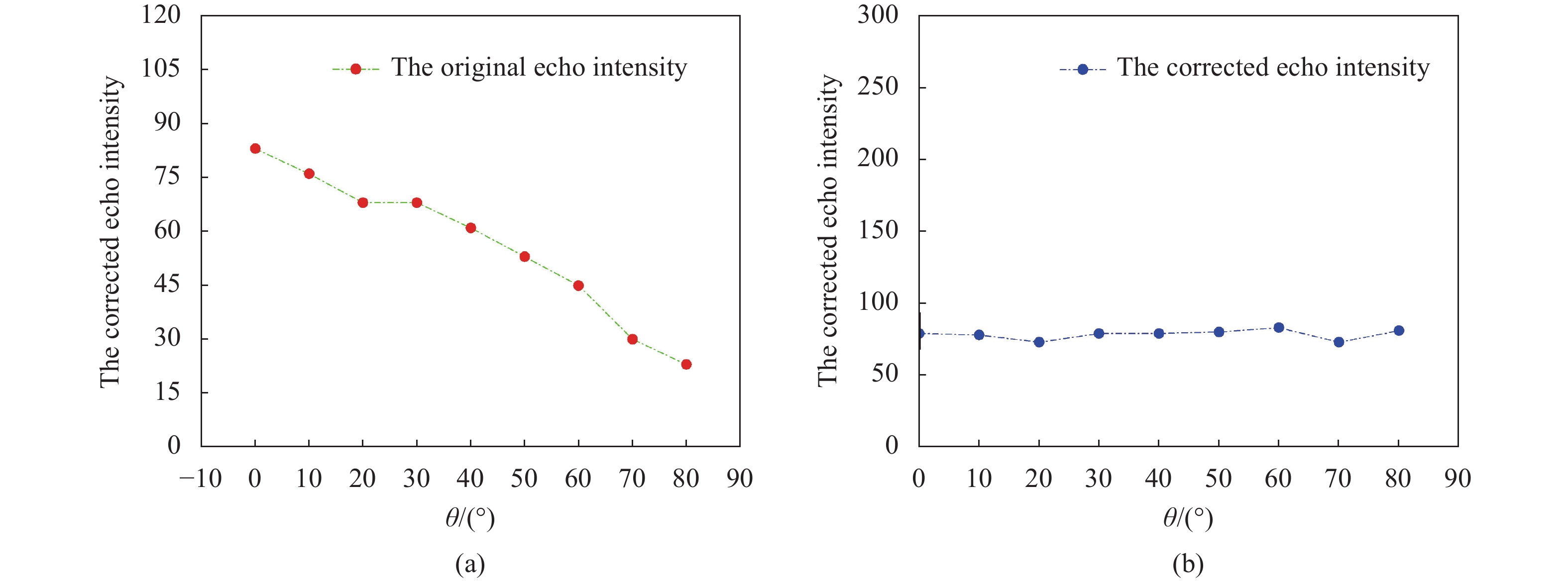
No. Specific expression 1 ${f}_{r}(R)=-24.116+61.2436\times {R}^{1}+3.6745\times {R}^{2}-2.0008\times {R}^{3}+0.1314\times {R}^{4},(R\leqslant 8.7\;\text {m})$ 2 $ {f}_{r}(R)=-7.993\times {10}^{3}+3.741\times {10}^{5}{(1/R)}^{1}-6.352\times {10}^{6}{(1/R)}^{2}+47.45\times {10}^{6}{(1/R)}^{3}-131.186\times {10}^{6}{(1/R)}^{4},(R > 8.7\;\text{m}) $ 3 ${f_\theta }(\cos \theta ) = 12.55 + 54.826 \times {(\cos \theta )^1} + 10.66 \times {(\cos \theta )^2}$ 由于不同厂商的激光雷达对回波强度的单位和数值尺度的表述并不一致,即便是来自同一厂商的不同激光雷达,在扫描同一目标时,回波强度值也会存在差异。表4中,分段多项式拟合校正函数的具体表达式仅适用于905 nm M8线阵激光雷达扫描获取的目标点云的强度数据,取${R_0}$=1.7 m,${\theta _0}$=0°,将${f_r}(R)$和${f_\theta }(\cos \theta )$代入公式(11)和公式(14)进行回波强度校正,95%标准漫反射板校正前后回波强度值分别如图15(a)、(b)和图16(a)、(b)所示。
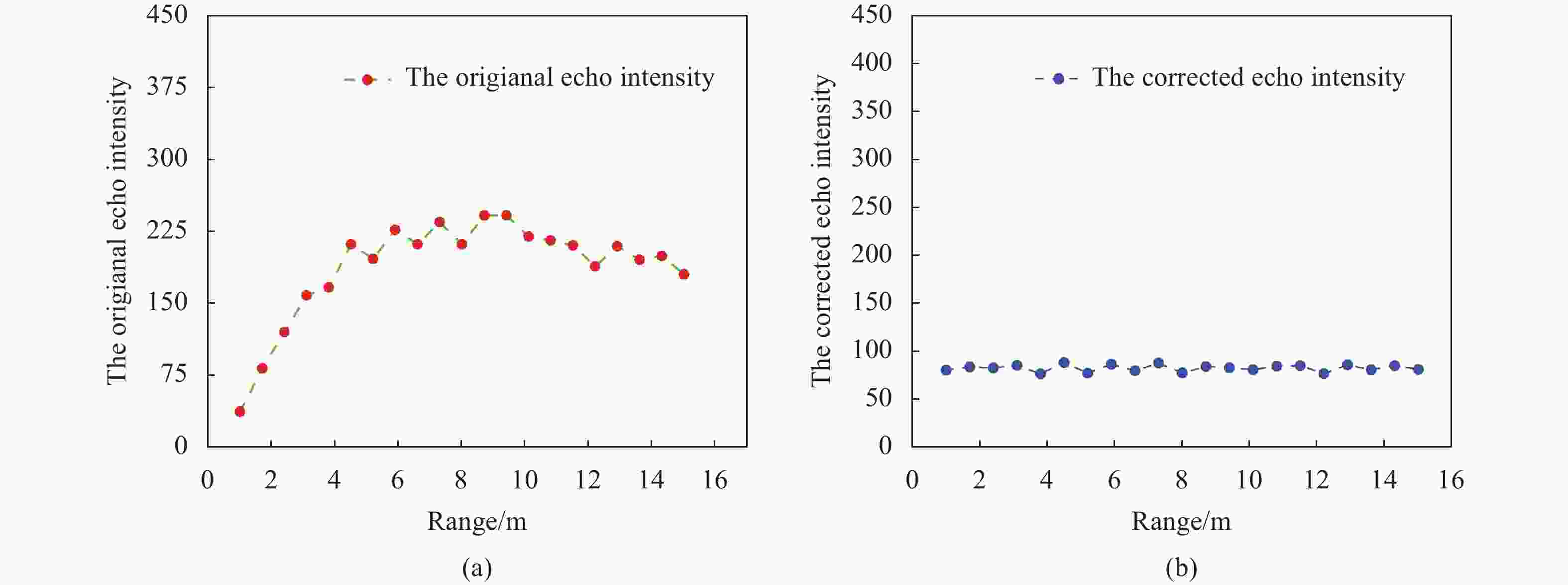
图 15 参考入射角为0°时距离影响下的原始强度 (a)及校正后强度 (b)
Figure 15. The original strength (a) and the corrected intensity (b) under the influence of distance when the reference incident angle is 0°

图 16 参考距离1.7 m时入射角影响下的原始强度 (a)及校正后强度 (b)
Figure 16. The original strength (a) and the corrected intensity (b) under the influence of incident angle when the reference distance is 1.7 m
-
从图15和图16可以看出,回波强度通过距离校正和入射角校正后,标准漫反射板的回波强度总体趋于一致。计算得到原始强度和校正之后的回波强度的最小值MIN,最大值MAX,平均值Mean以及标准差STD(Standard Deviation),如表5所示。
表 5 校正前后回波强度的最小值、最大值、平均值以及标准差
Table 5. The minimum, maximum, mean and standard deviation of the echo intensity before and after correction
Correction mode MIN MAX Mean STD Distanc effect
correctionOriginal 38 242 189 50.58 Corrected 77 89 83 3.49 Incidence angle effect
correctionOriginal 23 83 56 19.25 Corrected 72 82 77 3.17 从表5可以看出,校正前后距离影响下的回波强度标准差STD从50.58降低到了3.49,入射角影响下的回波强度标准差STD从19.25降低到了3.17。
为了更直观地显示强度校正效果,用变异系数(Coefficient of Variation, CV)表示强度校正前后的离散化程度大小,定义为:
$$ {{CV}} = \frac{{{{STD}}}}{{{{Mean}}}} \times 100\% $$ (19) 将校正后回波强度的变异系数CVCo与原始回波强度变异系数CVOr相比:
$$ \eta = \frac{{{{C}}{{{V}}_{{\text{Co}}}}}}{{{{C}}{{{V}}_{{\text{Or}}}}}} $$ (20) $ \eta $小于1时,表明校正后强度值的变异系数小于原始强度值,即强度校正模型具有有效性,$ \eta $越小,校正效果越好,校正前后回波强度一致性提升越高。
从表6可以看出,通过距离校正模型校正后的强度值变异系数CV从0.2676降低至0.0420,入射角校正模型校正后的强度值变异系数CV从0.3438降低至0.0412,回波强度的一致性分别提高了84.31%和88.02%。
表 6 校正前后回波强度变异系数CV及评价指标η和强度一致性
Table 6. CV of the echo intensity before and after correction and η and intensity consistency
Correction mode CV η Intensity consistency Distanc effect
correctionOriginal 0.2676 0.1569 84.31% Corrected 0.0420 Incidence angle effect
correctionOriginal 0.3438 0.1198 88.02% Corrected 0.0412 通过3.1节参考距离标定试验可知,强度值在1.7 m条件下能够真实地反映出目标的光谱反射特性,即1.7 m下的95%标准漫反射板的强度值代表真实的反射率95%,故将校正后的回波强度值均转化为反射率值,如图17所示。

图 17 不同距离角度下标准反射板(95%)的测量结果
Figure 17. The measurement results of standard reflector (95%) at different distance angles
-
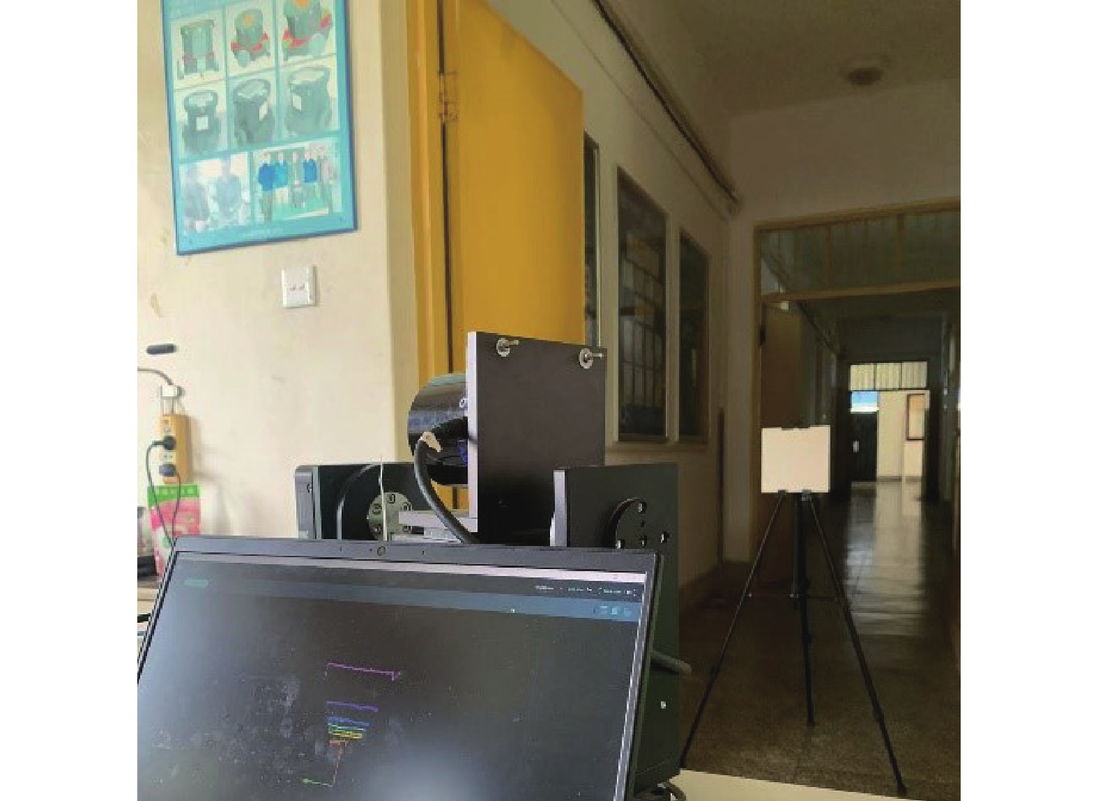
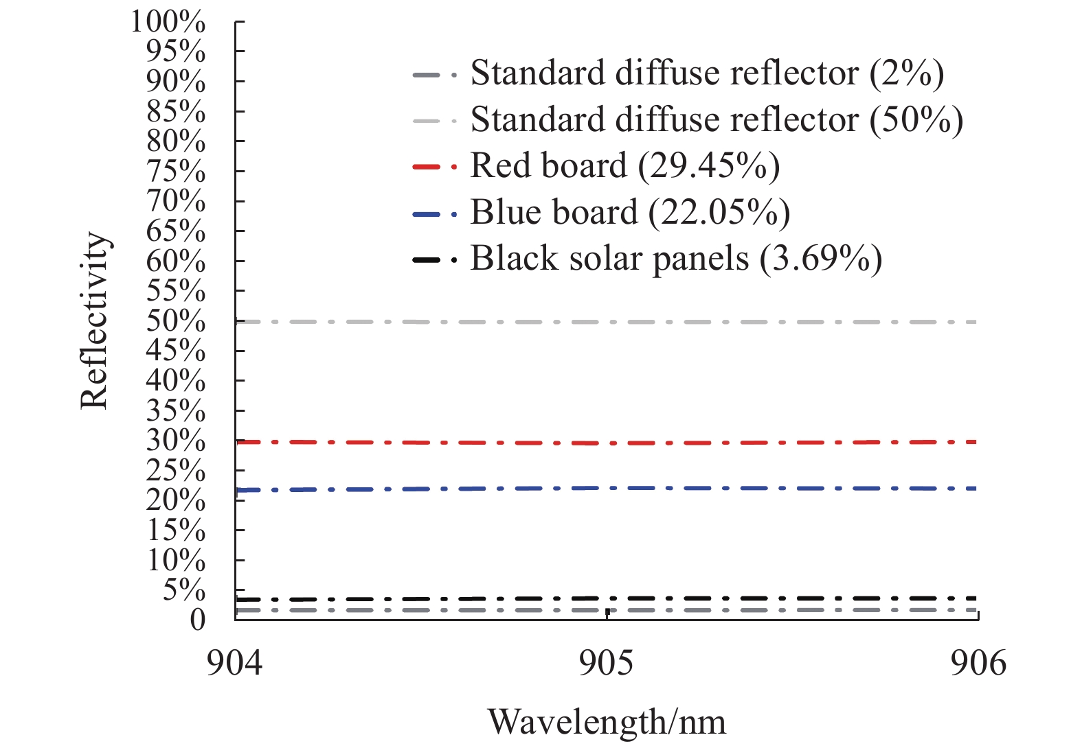
选取带有905 nm波段下反射率真值贴片的卫星模型进行三组发射率三维分布测量试验,卫星模型如图18所示,各贴片在905 nm波段下的反射率如图19所示,通过905 nm线阵激光雷达对目标模型进行线阵扫描,测量环境如图20所示。通过905 nm线阵激光雷达对目标模型进行线阵扫描,得到带有强度信息的卫星模型三维点云像,由于激光雷达易受到距离、入射角等因素的影响,卫星模型表面贴片所测得的强度值无法真实地反映每块贴片的反射光谱特性。测量出每块贴片中心的激光测距值R和每块贴片相对于激光雷达相对入射角度$\theta $,按照提出的强度校正模型对各部分贴片的强度数据进行校正,使各部分贴片所测得强度值能够真实反映各部分的反射光谱特性,将校正后的强度值转化为反射率。

图 18 卫星模型表面贴片分布
Figure 18. Surface patch distribution of satellite model

图 19 各贴片在905 nm下反射率真值
Figure 19. The true value of reflectivity of each patch at 905 nm

图 20 测量环境
Figure 20. The measuring environment
对于与环境处于热平衡状态的不透明表面来说,发射率等于吸收率,与反射率相加为1[21]。有公式(21):
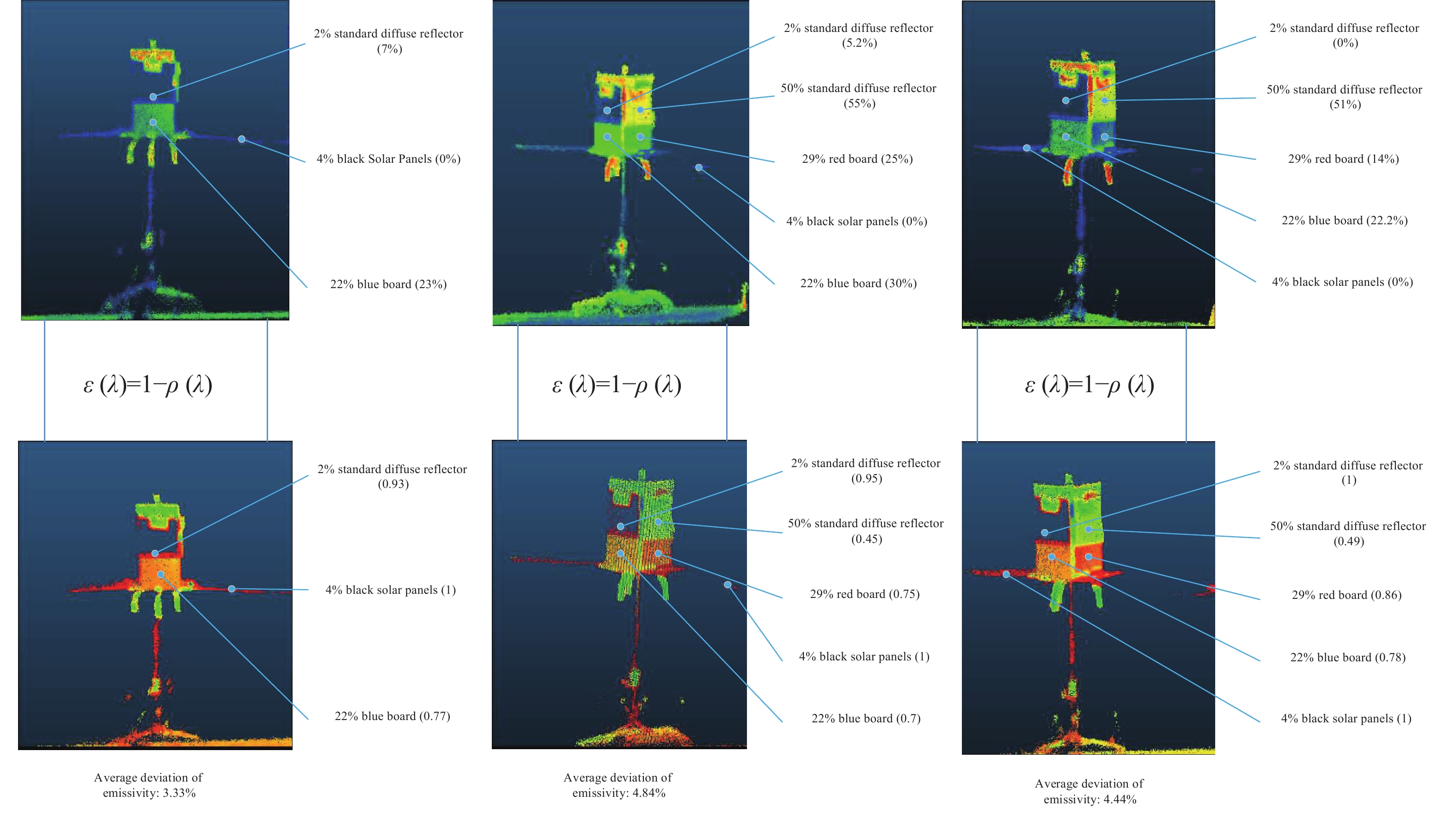
$$ \varepsilon (\lambda ) = 1 - \rho (\lambda ) $$ (21) 式中:$\varepsilon (\lambda )$为待测样品在波长$ \lambda $处的发射率;$\rho (\lambda )$为待测样品在波长$\lambda $处反射率。根据公式(21)求得目标模型贴片的反射率后便可进一步推导其表面发射率,得到目标模型表面的发射率三维分布,如图21所示。卫星模型表面贴片的发射率平均偏差均分别能控制在3.33%、4.84%和4.44%,如表7所示,为目标识别、低空可探测技术等提供技术支持。

图 21 卫星模型表面贴片发射率三维分布
Figure 21. Three-dimensional distribution of surface patch emissivity of satellite model
表 7 发射率平均偏差
Table 7. Average deviation of emissivity
Group 2% standard(0.98) 50% standard(0.5) 22% blue(0.78) 29% red(0.71) 4% solar array(0.96) Mean deviation 1 0.93 - 0.77 - 1 3.33% 2 0.95 0.45 0.70 0.75 1 4.84% 3 1 0.49 0.78 0.86 1 4.44% -
针对目前发射率测量方法大都只是对某一单一物质进行接触式测量,无法对复杂目标进行发射率三维分布测量的问题,基于M8激光回波提出了一种非接触式发射率三维分布测量方法。通过M8线阵激光雷达对95%标准漫反射板进行线阵扫描,得到具有反射光谱特性的雷达强度三维点云像;基于分段多项式模型校正距离和入射角度影响下的回波强度,验证强度校正模型的有效性;最后采用分段多项式校正模型对带有反射率真值贴片的缩比卫星模型雷达强度三维点云像进行强度校正,利用校正后的回波强度的反射光谱特性计算出目标表面的反射率,运用反射法进一步推导其发射率,得到缩比卫星模型发射率的三维分布,实现非接触式目标发射率三维分布测量。
文中采用的M8线阵激光雷达的波段为905 nm,属于红外波段中的近红外波段,暂无法涉及到中长红外波段的发射率测量,且所用材料反射率均为在室温条件下的真值,暂未涉及温度对发射率测量的影响。此外,由于不同激光雷达的物理因素差异以及对回波强度的单位和数值尺度的表述并不一致,即回波强度测量与校正部分仅适用特定的扫描仪器,但整体的测量流程思路仍具有一定的普适性。该发射率测量方法的鲁棒性和普适性还值得深入讨论,因此,下一步工作将进一步完善该方法的普适性及引入温度对发射率测量的相关影响。
Non-contact three-dimensional emissivity distribution measurement method of M8 LiDAR echo
-
摘要: 针对目前发射率测量方法只是对某一单一物质进行接触式测量,难以获得复杂目标的发射率三维分布问题,提出一种基于M8激光雷达回波的非接触式发射率三维分布测量方法。首先基于激光雷达传输距离方程分析回波强度特性,通过M8激光雷达对95%标准漫反射板进行扫描,叠加多帧单线点云,得到具有反射光谱特性的雷达强度三维点云像;运用分段多项式模型拟合距离-强度及入射角-强度之间的关系,基于得到的分段多项式模型校正距离和入射角度影响下的回波强度,使不同距离与入射角情况下所测回波强度能够真实地反映目标的反射光谱特性,校正结果显示,标准漫反射板回波强度变异系数分别从0.2676和0.3438降低到了0.0420和0.0412,回波强度一致性分别提高了84.31%和88.02%,使雷达所测得强度值能直接反映目标材料的反射光谱特性,验证了强度校正模型的有效性;最后基于得到的分段多项式校正模型对带有反射率真值贴片的缩比卫星模型雷达强度三维点云像进行强度校正,利用校正后的回波强度的反射光谱特性,计算出目标表面的反射率,运用反射法进一步推导其发射率,得到缩比卫星模型发射率的三维分布,三组卫星模型表面贴片的发射率平均偏差均分别能控制在3.33%、4.84%和4.44%。为目标识别、低空可探测技术等提供技术支持。Abstract:
Objective Emissivity is an important physical quantity to characterize the radiation ability of material surface. It is an important thermal physical parameter and has very important applications in many fields. Emissivity is not the intrinsic property of an object. It is a physical quantity that is difficult to measure accurately. It is related to temperature, wavelength, angle and so on. Its measurement is more complicated. At present, most of the emissivity measurement methods are only contact measurement of a single substance. It is impossible to measure the three-dimensional distribution of emissivity of complex targets. Combined with the characteristics of LiDAR, a non-contact three-dimensional distribution measurement method of emissivity is proposed based on LiDAR echo. Methods Firstly, the echo intensity characteristics are analyzed based on the LiDAR transmission distance equation, the main factors affecting the LiDAR echo intensity are explored, and the target point cloud data with intensity information by line array scanning of 95% reflectivity standard diffuse reflector plate are obtained by line array LiDAR (Fig.4). The stacked multi-frame single line point cloud (Fig.5) and the three-dimensional point cloud image of radar intensity with reflective spectral characteristics is obtained (Fig.8). Secondly, the piecewise polynomial model is used to fit the relationship between distance-intensity and incident angle-intensity (Tab.4). Based on the obtained piecewise polynomial model, the echo intensity under the influence of distance and incident angle is corrected, so that the measured echo intensity under different distance and incident angle can truly reflect the reflection spectrum characteristics of the target, and the validity of the correction model is verified (Fig.15-16). Finally, based on the obtained piecewise polynomial correction model, the intensity correction of the three-dimensional point cloud image of the radar intensity of the scaled satellite model with the reflectivity true value patch is carried out. The reflectivity of the target surface is calculated by using the reflectance spectral characteristics of the corrected echo intensity. The emissivity is further deduced by the reflection method, and the three-dimensional distribution of the emissivity of the scaled satellite model is obtained (Fig.21). Results and Discussions The correction results show that the standard deviation of echo intensity STD under the influence of distance before and after standard diffuse reflection correction is reduced from 50.58 to 3.49 (Tab.5), and the standard deviation of echo intensity STD under the influence of incident angle is reduced from 19.25 to 3.17 (Tab.5). The coefficient of variation of echo intensity under the influence of standard diffuse reflection plate distance effect and incident angle effect is reduced from 0.267 6 and 0.343 8 to 0.042 0 and 0.041 2 (Tab.5) respectively. And the consistency of echo intensity is increased by 84.31% and 88.02% respectively (Tab.6). The average emissivity deviations of the surface patches of the three satellite models can be controlled at 3.33%, 4.84% and 4.44%, respectively (Tab.7). Conclusions In view of the fact that most of the current emissivity measurement methods are only contact measurement of a single substance, it is impossible to measure the three-dimensional distribution of emissivity of complex targets. Combined with the characteristics of LiDAR, a non-contact emissivity three-dimensional distribution measurement method is proposed based on M8 LiDAR echo. The band of the M8 linear array LiDAR used in this paper is 905 nm, which belongs to the near-infrared band in the infrared band, and the emissivity measurement in the medium and long infrared band cannot be involved. The reflectivity of the materials used in this paper is the true value at room temperature, and the influence of temperature on emissivity measurement is not involved. In addition, due to the differences in physical factors of different LiDARs and the inconsistent expression of the unit and numerical scale of the echo intensity, the current measurement method is only applicable to specific scanning instruments. The robustness and universality of the emissivity measurement method are worthy of further discussion. Therefore, the next step will further improve the universality of the method and introduce the influence of temperature on the emissivity measurement. -
Key words:
- LiDAR /
- emissivity /
- reflectivity /
- echo intensity /
- echo intensity correction
-
图 10 参考入射角0°时1~15 m强度测量示意图
Figure 10. Strength measurements at different positions of 1-15 m at a reference incident angle of 0°
图 11 参考入射角0°时1~15 m强度测量场景图
Figure 11. Referring to the real scene of 1-15 m intensity measurement at the incident angle of 0°
图 12 参考入射角0°时雷达测距值与回波强度的关系
Figure 12. The relationship between LiDAR ranging value and echo intensity when the reference incident angle is 0°
图 13 参考距离1.7 m时入射角0°~80°的强度测量
Figure 13. Intensity measurement at different sites of 0°-80° at areference distance of 1.7 m
图 14 参考距离为1.7 m时雷达入射角与回波强度的关系
Figure 14. The relationship between LiDAR incident angle and echo intensity when the reference distance is 1.7 m
图 15 参考入射角为0°时距离影响下的原始强度 (a)及校正后强度 (b)
Figure 15. The original strength (a) and the corrected intensity (b) under the influence of distance when the reference incident angle is 0°
图 16 参考距离1.7 m时入射角影响下的原始强度 (a)及校正后强度 (b)
Figure 16. The original strength (a) and the corrected intensity (b) under the influence of incident angle when the reference distance is 1.7 m
图 17 不同距离角度下标准反射板(95%)的测量结果
Figure 17. The measurement results of standard reflector (95%) at different distance angles
图 19 各贴片在905 nm下反射率真值
Figure 19. The true value of reflectivity of each patch at 905 nm
图 21 卫星模型表面贴片发射率三维分布
Figure 21. Three-dimensional distribution of surface patch emissivity of satellite model
表 1 不同距离下标定样板的强度值
Table 1. Strength value of the calibration template at different distances
Group 95% 50% 2% Blue
(22%)Green
(18%)White
(62%)Black
(4%)0.5 m 8 8 0 0 0 8 0 1.0 m 38 23 0 0 0 30 0 1.5 m 68 45 0 15 8 23 0 1.7 m 83 45 0 23 23 45 0 2.0 m 91 68 0 61 61 77 15 2.4 m 121 98 0 98 76 122 76 3.1 m 159 136 0 121 128 151 113  下载: 导出CSV
表 2 不同阶数下多项式拟合函数均方根误差
Table 2. Root mean square error of polynomial fitting function under different orders
Order RMSE K M N 1 26.34 8.42 2.84 2 11.92 7.65 2.76 3 10.06 7.28 2.73 4 9.65 5.98 1.96 5 9.44 5.98 1.86 6 9.17 5.90 0.89
下载: 导出CSV
表 3 各个多项式系数
Table 3. Coefficients of each polynomial
Coefficient Value ${a_0}$ −24.116 ${a_1}$ 61.2436 $ {a_2} $ 3.6745 ${a_3}$ −2.0008 $ {a_4} $ 0.1314 ${b_0}$ −7.993×10³ ${b_1}$ 3.741×10⁵ ${b_2}$ −6.352×10⁶ ${b_3}$ 47.45×10⁶ ${b_4}$ −131.186×10⁶ ${c_0}$ 12.5477 ${c_1}$ 54.826 ${c_2}$ 10.66
下载: 导出CSV
表 4 分段多项式拟合校正函数的具体表达式
Table 4. Specific expression of the distance and incident angle cosine polynomial correction function
No. Specific expression 1 ${f}_{r}(R)=-24.116+61.2436\times {R}^{1}+3.6745\times {R}^{2}-2.0008\times {R}^{3}+0.1314\times {R}^{4},(R\leqslant 8.7\;\text {m})$ 2 $ {f}_{r}(R)=-7.993\times {10}^{3}+3.741\times {10}^{5}{(1/R)}^{1}-6.352\times {10}^{6}{(1/R)}^{2}+47.45\times {10}^{6}{(1/R)}^{3}-131.186\times {10}^{6}{(1/R)}^{4},(R > 8.7\;\text{m}) $ 3 ${f_\theta }(\cos \theta ) = 12.55 + 54.826 \times {(\cos \theta )^1} + 10.66 \times {(\cos \theta )^2}$
下载: 导出CSV
表 5 校正前后回波强度的最小值、最大值、平均值以及标准差
Table 5. The minimum, maximum, mean and standard deviation of the echo intensity before and after correction
Correction mode MIN MAX Mean STD Distanc effect
correctionOriginal 38 242 189 50.58 Corrected 77 89 83 3.49 Incidence angle effect
correctionOriginal 23 83 56 19.25 Corrected 72 82 77 3.17
下载: 导出CSV
表 6 校正前后回波强度变异系数CV及评价指标η和强度一致性
Table 6. CV of the echo intensity before and after correction and η and intensity consistency
Correction mode CV η Intensity consistency Distanc effect
correctionOriginal 0.2676 0.1569 84.31% Corrected 0.0420 Incidence angle effect
correctionOriginal 0.3438 0.1198 88.02% Corrected 0.0412
下载: 导出CSV
表 7 发射率平均偏差
Table 7. Average deviation of emissivity
Group 2% standard(0.98) 50% standard(0.5) 22% blue(0.78) 29% red(0.71) 4% solar array(0.96) Mean deviation 1 0.93 - 0.77 - 1 3.33% 2 0.95 0.45 0.70 0.75 1 4.84% 3 1 0.49 0.78 0.86 1 4.44%
下载: 导出CSV
-
[1] 曹飞飞, 吉洪湖, 于明飞, 等. 低发射率材料涂敷区域对排气系统壁温和红外特性的影响 [J]. 红外与激光工程, 2020, 49(10): 20190131-95. Cao Feifei, Ji Honghu, Yu Mingfei, et al. Effects of low emissivity material coating site onwall temperature and infrared characteristics of exhaust system [J]. Infrared and Laser Engineering, 2020, 49(10): 20190131. (in Chinese) [2] 戴景民, 王新北. 材料发射率测量技术及其应用 [J]. 计量学报, 2007(3): 232-236. Dai Jingmin, Wang Xinbei. Review of emissivity measurement and its applications [J]. Acta Metrologica Sinica, 2007(3): 232-236. (in Chinese) [3] 傅莉, 樊金浩, 张兆义, 等. 双向反射分布函数结合Bi-LSTM网络求解壁面发射率 [J]. 红外与激光工程, 2023, 52(2): 20220355. doi: 10.3788/IRLA20220355 Fu Li, Fan Jinhao, Zhang Zhaoyi, et al. Wall emissivity solved by bidirectional reflection distribution function combined with Bi-LSTM network [J]. Infrared and Laser Engineering, 2023, 52(2): 20220355. (in Chinese) doi: 10.3788/IRLA20220355 [4] 徐记伟, 周军. 毫米波迷彩隐身涂层发射率分布数值计算 [J]. 红外与激光工程, 2017, 46(3): 321002-0321002(5). Xu Jiwei, Zhou Jun. Numerical calculation of millimeter wave pattern painting stealthy coat emissivity [J]. Infrared and Laser Engineering, 2017, 46(3): 0321002. (in Chinese) [5] Le V T, Goo N S. Design, Fabrication, and testing of metallic thermal protection systems for spaceplane vehicles [J]. Journal of Spacecraft and Rockets, 2021, 58(2): 1-18. doi: 10.2514/1.A34908 [6] Iuchi T, Furukawa T. Emissivity-compensated radiation thermometry [C]//International Measurement Confederation World Congress, 2000, 1065: 122008. [7] Adachi M, Hamaya S, Yamagata Y, et al. In-situ observation of AlN formation from Ni-Al solution using an electromagnetic levitation technique [J]. Journal of the American Ceramic Society, 2020, 103(4): 2389-2398. doi: 10.1111/jace.16960 [8] Adachi M, Sato A, Hamaya S, et al. Containerless measurements of the liquid-state density of Ni–Al alloys for use as turbine blade materials [J]. SN Applied Sciences, 2018, 1(1): 18. [9] Adachi M, Yamagata Y, Watanabe M, et al. Composition dependence of normal spectral emissivity of liquid Ni–Al alloys [J]. Iron and Steel Institute of Japan, 2021, 61(3): 684-689. [10] 丁经纬, 郝小鹏, 于坤, 等. 黑体涂层光谱发射率特性研究 [J]. 红外与激光工程, 2023, 52(10): 20230033. doi: 10.3788/IRLA20230033 Ding Jingwei, Hao Xiaopeng, Yu Kun, et al. Research on spectral emissivity characteristics of blackbody coatings [J]. Infrared and Laser Engineering, 2023, 52(10): 20230033. (in Chinese) doi: 10.3788/IRLA20230033 [11] Qi J, Eri Q, Kong B, et al . The radiative characteristics of inconel 718 superalloy after thermal oxidation [J]. Journal of Alloys and Compounds, 2021, 854(287): 156414. [12] Yu K, Tong R, Zhang K, et al. An apparatus for the directional spectral emissivity measurement in the near infrared band [J]. International Journal of Thermophysics, 2021, 42(6): 1-15. doi: 10.1007/s10765-021-02813-0 [13] Xu Y, Zhang K, Yu K, et al. Temperature-dependent emissivity models of aeronautical alloy DD6 and modified function for emissivity computation with different roughness [J]. International Journal of Thermophysics, 2021, 42(1): 1-21. doi: 10.1007/s10765-020-02754-0 [14] 袁良, 袁林光, 董再天, et al. 高温状态下的材料法向光谱发射率测量 [J]. 应用光学, 2023, 44(3): 33-39. doi: 10.5768/JAO202344.0303002 Yuan Liang, Yuan Linguang, Dong Zaitian, et al. Measurement of normal spectral emissivity of materials at high temperature [J]. Journal of Applied Optics, 2023, 44(3): 33-39. (in Chinese) doi: 10.5768/JAO202344.0303002 [15] Ding Qiong, Yu Junpeng. LiDAR intensity calibration based on multiple strips [J]. Remote Sensing Information, 2018, 33(5): 89-93. (in Chinese) doi: 10.3969/j.issn.1000-3177.2018.05.014 Ding Qiong, Yu Junpeng. LiDAR intensity calibration based on multiple strips [J]. Remote Sensing Information, 2018, 33(5): 89-93. (in Chinese) doi: 10.3969/j.issn.1000-3177.2018.05.014 [16] Sanna K, Anttoni J, Mikko K, et al. Analysis of incidence angle and distance effects on terrestrial laser scanner intensity: search for correction methods [J]. Remote Sensing, 2011, 3(10): 2207-2221. doi: 10.3390/rs3102207 [17] Ferrero A, Rabal A M, Campos J, et al. Spectral and geometrical variation of the bidirectional reflectance distribution function of diffuse reflectance standards[J]. Applied Optics , 2012, 51(36): 8535-8540. [18] Coren F, Sterzai P. Radiometric correction in laser scanning [J]. International Journal of Remote Sensing, 2006, 27(15): 3097-3104. doi: 10.1080/01431160500217277 [19] Perez D, Quintana Y. A survey on the Weierstrass approximation theorem [J]. Divulgaciones Matematicas, 2008, 16(1): 231-247. [20] Tan K, Chen X. Correction of incidence angle and distance effects on TLS intensity data based on reference targets [J]. Remote Sensing, 2016, 8(3): 251. doi: 10.3390/rs8030251 [21] Wang C, Hu J, Wang F, et al. Measurement of Ti–6Al–4V alloy ignition temperature by reflectivity detection [J]. Review of Scientific Instruments, 2018, 89(4): 044902. doi: 10.1063/1.5019241 -

 点击查看大图

计量
- 文章访问数: 13
- HTML全文浏览量: 17
- PDF下载量: 2
- 被引次数: 0

