


 下载:
下载:


-
激光通信是以激光作为信息的载波在大气空间传输的一种通信方式。除了时分复用、波分复用等,激光通信系统可采用模分复用、偏振复用等方式,使得通信信道容量倍增,因此受到了较多的关注[1−4]。通过对振幅、相位、偏振、轨道角动量等自由度进行多维调制[5−8],激光通信的信道容量还有进一步提升的空间。同时,激光通信还具有体积小、安全性好等特点[9−11]。虽然星地激光通信性能较优,但受大气湍流的影响较大[12−16]。大气湍流空间分布的非均匀性会使得其中传输的光束产生波前畸变,产生光束漂移、光强闪烁等现象。描述大气湍流对光线影响的参数主要有大气折射率结构常数、视宁度、大气相干长度、大气相干时间、等晕角等。在激光通信系统中,大气湍流提升了系统的误比特率,降低了通信质量[17−21]。在中等及弱湍流条件下,自适应光学可以显著提高数据传输链路的性能,但在强湍流条件下,其能力仍然有限[22],故星地激光通信链路通常工作在中等强度或弱湍流条件下,以确保通信质量[23−24]。预测大气湍流可以提前对星地数据传输链路进行调度,以及预先部署自适应光学方案来补偿湍流效应,避免建立无效的通信任务或减轻大气湍流造成的数据传输链路性能退化,因此大气湍流预报对于星地激光通信至关重要。此外,大气光学湍流预报研究在其他领域也具有重要的科学研究意义和工程应用价值,为天文观测与选址、光学遥感等提供关键参数。
文中主要综述了现阶段常见的几种大气湍流预测技术,主要包括:较为成熟与广泛应用的中尺度数值预报方案、不依赖经验公式的深度学习预报方案、提升短时预报精度的变模态分解预报方案等。
-
由于大气湍流的复杂性以及计算机的算力限制,直接数值求解大气光学湍流问题短期内较难实现,通过建立中尺度数值预报输出的常规气象参数,再采用湍流参数化方案建立常规气象参数与光学湍流特征量的关系来预报大气光学湍流是目前较为可行的解决方案。中尺度数值预报经过数十年的发展已经逐步走向成熟,在全球得到广泛应用,代表性的中尺度气象模式[25−27]包括 Meso-Nh (Non-hydrostatic mesoscale atmospheric model), MM5 (Mesoscale Model 5), WRF (Weather Research & Forecasting Model)和 Polar WRF 等。国内外在光学湍流参数化的方案[28−31]上也已有较多成果,这类模型通常是基于大量观测数据,并在基础上总结出的$ {C}_{n}^{2} $廓线模式经验公式,其结果为统计均值。常见的光学湍流参数化方案包括Hufmagel模型[28]、Tatarski模型[29]等,参数包含高度及其他常规气象参数。
1986年,Coulman et al.最先提出从预报的常规气象参数中获取大气湍流参数的方法[32],并将该方法得到的数据与AAT(Anglo Australian Telescope)实地观测得到的大气视宁度数据进行对比。结果表明,在视宁度小于2"时,二者有一定的相关性。1999年,Masciadri等在大气光学湍流数值模型研究方面取得了进展,以ECMWF的分析资料和探空雷达数据作为初始场,采用Meso-NH模式对Cerro Paranal台址进行气象参数和大气湍流预报,计算出了Cerro Paranal台址周围压强、温度、风速和大气湍流强度廓线,模型计算结果与实测$ {C}_{n}^{2} $廓线的对比如图1(a) 所示[33−34]。在此基础上,通过积分进一步计算了视宁度、大气相干时间、等晕角、闪烁率和湍流外尺度的结果,计算结果水平分辨率为500 m,近地面垂直分辨率为50 m,随着高度上升分辨率逐步增加到600 m。Cheinet 和Beljaars通过欧洲中期天气预报中心 (ECMWF)的综合预报系统预报出分辨率1°×1°的经纬度网格上的常规气象参数,结合湍流参数化方案计算出近地面$ {C}_{n}^{2} $,显示出了近地面$ {C}_{n}^{2} $的季节变化特征以及区域特征[35]。
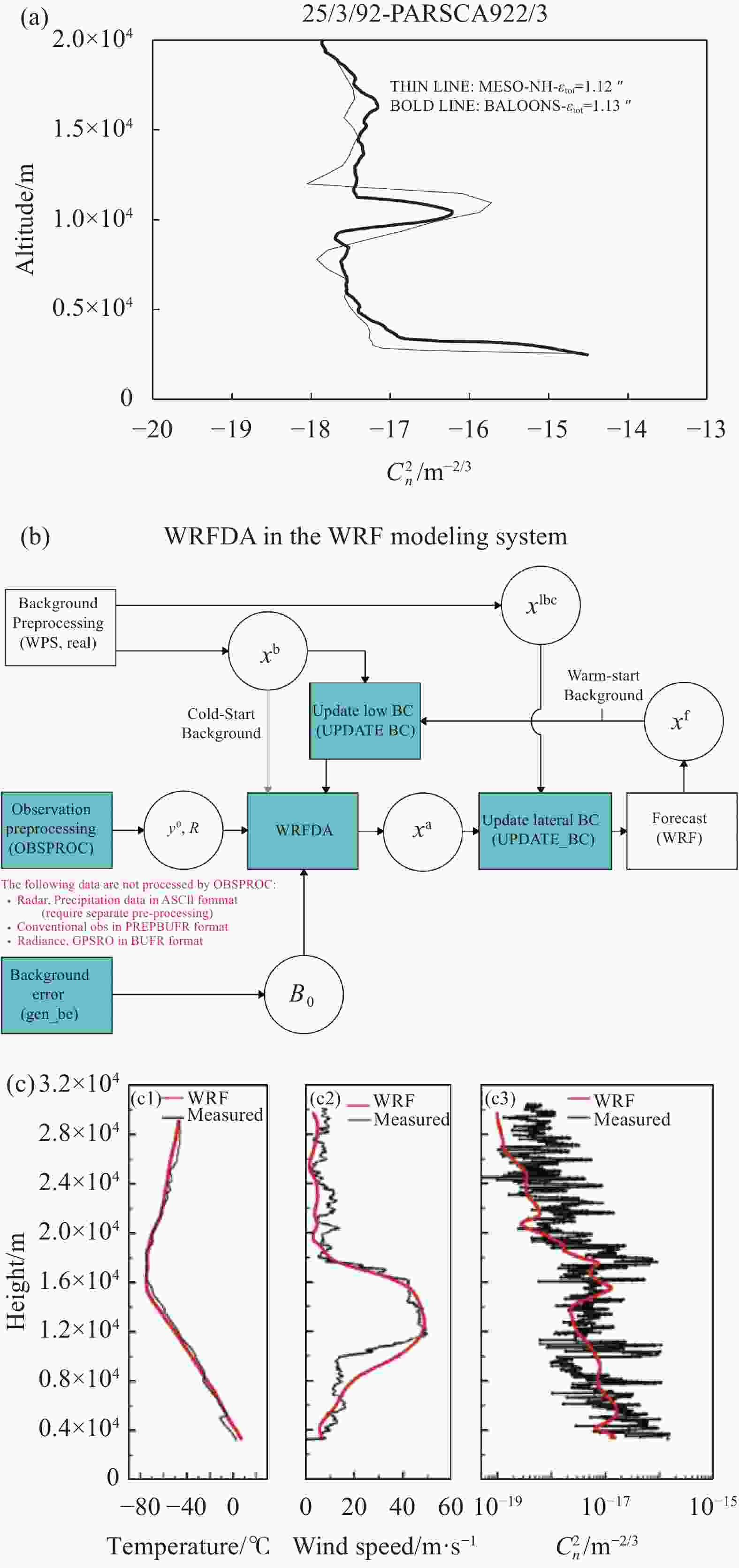
图 1 大气湍流的中尺度数值预报。(a) Cerro Paranal台址模型计算结果与实测$ {C}_{n}^{2} $廓线的对比[33];(b) WRF预报系统工作流程图[25];(c) 高美古WRF预报结果与实测结果的比较
Figure 1. The meso-scale numerical prediction of atmosphere turbulence. (a) Results comparison between the model of Cerro Paranal station site and the measured $ {C}_{n}^{2} $ profiles[33]; (b) WRF modeling system flow chart[25]; (c) Comparison of WRF and measured data at Gaomeigu
在众多中尺度数值预报模式中,WRF模式应用最为广泛。该模式由美国大气研究中心(NCAR)、国家环境预报中心 (NCEP)等多单位联合研制,由 NCAR的MM5模式发展而来。与MM5相比,WRF模式在算法和软件框
架设计、动力模块、硬件平台适配性、应用范围、数据格式、可移植等方面更具优势,其模式程序编写的标准化、动力框架与物理方案等功能的模块化以及模式程序的并行化使模式程序能够更好的适应新型计算平台,更符合新一代气象数值预报模式的总体要求。自2000年初推出第一个版本以来,WRF目前已更新至4.5版本,工作流程如图 1(b) 所示。WRF模型初始化阶段会收集实时气象观测数据和地球物理场信息,并应用数据同化方法以构建初始场。随后在模型配置阶段,根据研究或预报的具体需求,设定适宜的模拟时间跨度、空间分辨率和物理参数化选项。完成这些设置后,模型进入运行阶段,此时,WRF通过其动力学核心与物理参数化模块,对大气状态进行数值模拟,以推进时间维度的天气预报。基于WRF的大气湍流预报工作也日渐丰富,并在天文选址等领域开始应用。
1999年,Cherubini等[36]基于夏威夷大学的Mauna Kea气象中心的平台,对夏威夷Mauna Kea天文台进行常规气象参数预报;2008年,Cherubini[37−38]选用中尺度MM5模式预报了Mauna Kea天文台近地面的$ {C}_{n}^{2} $,采用的大气光学湍流模型以及校准方法与Masc-iadri方法一致,但在垂直分辨率等方面有所不同。自MM5从2005年停止更新后,转为使用WRF模式。Mahalov and Moustaoui[39]将微尺度模式耦合到WRF模式从而模拟高对流层和低平流层的$ {C}_{n}^{2} $,该方案以WRF输出产品作为微尺度模式的初始场和边界条件,WRF预报水平格距为1 km,垂直格距为150 m。Lascaux [40]等将中尺度数值预报 $ {C}_{n}^{2} $廓线和视宁度的方法应用到在南极的天文选址工作中。
大气湍流模型有一定地域性,没有通用公式与方法能满足我国复杂的自然地理情况,因此,针对实际的地理情况与气象情况对大气湍流预报模型不断调整,完善出适合我国环境的大气湍流预报方案有重要意义。虽然我国开展大气湍流预报的研究相对较晚,但也积累了一定的阶段性成果。中国科学院安徽光学精密机械研究所在大气湍流模型研究方面积累了多年的工作基础,在全国多个区域开展了一系列的$ {C}_{n}^{2} $廓线地面实测工作,对合肥、兴隆、昆明、东山和库尔勒等地的平均$ {C}_{n}^{2} $廓线公式进行了拟合[41−43]。2007年,吴晓庆等提出利用中尺度气象模式方法对大气湍流进行预报[44];2008年,许利明等采用MM5气象模式和Dewan模型,对合肥、库尔勒和东山三地的$ {C}_{n}^{2} $廓线进行了预报,$ {C}_{n}^{2} $廓线预报结果与大气湍流廓线的一般特征相符[45]。随着WRF模式的快速发展,中国科学院安徽光学精密机械研究所Qing等通过 WRF模式,进一步研究预报高美古、茂名、库尔勒等典型地区的$ {C}_{n}^{2} $廓线,高美古地区预报结果如图1(c) 所示[46−47]。与探空气球实测的$ {C}_{n}^{2} $廓线相比,预报结果与实测值的整体趋势较为吻合,但是细节处存在一定差异。2016年,Qing等将WRF模式与Monin-Obukhov 理论结合,对中国南海近海面、中国南极泰山站冰雪面上以及成都地区近地面层的$ {C}_{n}^{2} $进行预报,取得了较好的效果,表明了基于WRF模式对近地面层$ {C}_{n}^{2} $进行预报的可行性[48−49]。2023年,中国科学院安徽光学精密机械研究所Qing等基于历史探测数据集和大数据融合分析技术,并耦合欧洲第五代大气再分析数据集,建立了全球大气光学湍流预测模型,其预测结果如图2所示。该方法突破了广域环境下大气光学湍流特征难以高效获取的局限,解决了广域大气光学湍流预测及可视化表征的关键科学与技术问题[50]。

大气湍流预报研究对我国的天文选址工作也有重要作用。从中尺度数值预报方法在天文选址上的重要性出发,国家天文台选址组自2010年开始对国内站址的大气湍流模型展开研究,以气象条件较好的兴隆站、高美古站和西藏的阿里候选站站址为研究对象,建立其大气湍流特征的模型。王红帅等选以 WRF 模式为基础估算大气湍流, 并将其应用于中国西部地区的天文选址工作[51−53]。2021年,国家天文台Qian等利用WRF模型结合Trinquet–Vernin参数化方法研究了西藏阿里天文台的大气湍流,发现阿里天文台具有良好的地面观测大气湍流条件的较大优势,特别是在夏季[54]。
-
近年来,深度学习方法在各领域中的应用得到了广泛关注[55]。深度神经网络可以学习到从输入数据到目标标签之间的映射关系,因此在各种任务中表现出色,例如语义分割[56−57]、医学图像处理[58−62]、数字全息[63−65]、计算成像[66−74]、超分辨[75−77]、图像识别[78−80]等。
深度学习在气象预报领域的探索由来已久。1992 年,French 等基于BP算法(Backpropagation Algori-thm)实现了对降雨量的时空场分布提前1 h的预报[81]。近年来,深度学习方法在气象预报上的能力不断增强。香港理工大学 Qiu等提出了一种基于多任务卷积神经网络的短期降水预报方法,并针对观测数据不完备和临界点对观测的影响,采用多个观测数据间的相关关系实现了降水短期预报,取得了比基线模型更好的效果[82]。2012 年,阿里巴巴集团Liu等将基于混沌神经网络(CONN)的方法应用于香港国际机场附近风剪切的预测研究中,利用CONN预报的多普勒速度可以转化为逆风廓线,进而识别风切变的发生[83]。2019年,北京信息科技大学孙全德等利用 LASSO回归、随机森林、深度学习等三种算法,改进了中尺度数值预报方法预报的华北地区中尺度10 m风速,相比传统方法取得了较好的效果[84]。2020年, Sonderby等人建立了基于深度学习的降雨预测模型 MetNet,可以提前7~8 h对美国境内范围进行了降水量预测,空间分辨率为1 km,时间分辨率为2 min。预报结果示例如图3所示,超过了 NOAA 使用的大气模型结果[85]。2023年,MetNet模型更新至MetNet-3,提供了一个时间更平滑且高度精细的预报,提前时间间隔为 2 min,空间分辨率为 1 ~ 4 km[86]。

随着深度学习方法的日渐成熟,国内外学者逐渐将其应用到由预报大气光学湍流的工作中。2016 年,北卡罗莱纳州立大学 Wang等利用多层感知机网络对夏威夷Mauna Loa天文台附近的近地面$ {C}_{n}^{2} $进行4周的预测[87]。网络结构如图4(a) 所示,输入取5个直接影响$ {C}_{n}^{2} $的常规气象参数,包括2 m 处温度、湿度、气压和 15 m 处位温梯度、风剪切,气象参数需要取5 min平均以平滑,输出为15 m处的$ {C}_{n}^{2} $。结果显示,在夜间大气条件较为良好的情况下,$ {C}_{n}^{2} $估算值偏高,但机器学习方法在捕捉$ {C}_{n}^{2} $的日变化特征以及各种近地面各种大气稳定性条件的适应性方面有较好的表现,该结果表明了利用深度学习的方法对大气湍流进行预报有较强的可行性。

图 4 基于深度学习的大气光学湍流预报方案。(a) BP算法网络结构[87];(b) AGA-BP 神经网络结构[89];(c)实测值、AGA-BP 网络预报值、Polar WRF预报值的比对结果[89]
Figure 4. Atmospheric optical turbulence prediction through deep learning. (a) BP neural network[87]; (b) AGA-BP neural network[89]; (c) Results of measured data, Polar WRF prediction, AGA-BP neural network prediction[89]
2017 年,中国科学院安徽光学精密机械研究所吕洁等基于BP神经网络和逐步回归理论,采用不同的因子分别建立光学湍流参数化模型,对三亚地区近海面 $ {C}_{n}^{2} $进行预报[88]。以温度、相对湿度、风速为BP网络输入参数,建立了反向传递神经网络;以温度、温度三次幂、相对湿度三次幂、温度平方与风速乘积,温度平方与风速平方乘积为逐步回归方法的输入。模型结果表明,两个模型方法在变化的趋势及量级上都与实测值相近,估计值与实测值的相关系数都大于0.8,但18:00以后的预测精度都不及日间。
2020年,中国科学院安徽光学精密机械研究所苏昶东等将自适应遗传算法 AGA(Adaptive Genetic Algorithm)与 BP算法的优势相结合,构建AGA-BP混合算法,将其用于南极泰山站的近地大气湍流预报,并与相似理论的梯度法、Polar WRF三种方法的预报结果进行对比。BP算法是一种梯度下降算法,它的目的是使模型的拟合精度达到最大,同时降低总体误差。但该方法的学习过程是从一个初始点开始,沿着误差函数的斜率逐步逼近其最小值,容易陷入局部最优等问题。在BP算法基础上,AGA-BP混合算法通过遗传算法生成输入 BP网络的初始权重分布和阈值,对BP算法效果有较大提升。对比使用的实测数据来自于南极泰山站,时间范围为2013-12-30—2014-02-10。模型结构如图4(b) 所示,输入为2 m以及0.5 m两层的气温、相对湿度、风速,以及地表面辐射温度,输出为地表大气光学湍流强度$ {C}_{n}^{2} $。预报结果如图4(c) 所示。结果显示,AGA-BP神经网络初步证明了,虽然总体训练数据规模有限,但在不含任何先验公式的情况下,该模型预测南极泰山站近地面的$ {C}_{n}^{2} $时间演化性能令人满意,可以相对可靠地估计出近地面的$ {C}_{n}^{2} $。
-
虽然通过光学湍流参数化方案预报大气湍流是目前主流的解决方案,但该方案准确性受到气象预报参数准确性的限制。中尺度数值模式的水平和垂直分辨率足以解决几十米的薄大气湍流层[90−92],但由于大气湍流的时空尺度远小于中尺度气象预报通常能达到的最高分辨率[93] ,使用WRF模式预测几小时内大气湍流的精度难以让人满意[94]。此外,无论由于参数化湍流方案主要是基于一些假设,根据历史数据和经验总结而来,无论是经验模式还是物理模式,都难以准确描述气象参数与大气湍流之间的关系[95],大多只针对特定条件和位置开发[96],在某些特定条件下的适用性不尽人意。近年来,一些优秀的深度学习算法被用于建立预报模型,显示出了深度学习较强的泛化能力[97] ,尽管其预报精度仍然受到气象预报数据准确性的限制。在激光通信领域,分析描述大气湍流强度特征。最相关和常用的参数是大气相干长度$ {r}_{0} $,大气相干长度$ {r}_{0} $是湍流强度在传输路径上的积分值,也可用于计算大气湍流参数如视场和闪烁指数。
最近,笔者课题组联合中国科学院空天信息创新研究院与提出了一种基于变分模态分解和自回归模型的混合模型(TsVMD-AR),可以提高短期大气湍流预报的能力[98]。数据集为差分像视宁度监视仪采集的2021-12-02—2022-01-05、2022-1-10—2022-01-25、2022-05-01—2022-05-15的实测大气相干长度数据,预测的准确性用平均绝对误差(MAE)、平均绝对百分比误差(MAPE)和均方根误差(RMSE)来评估。首先,使用变分模态分解(VMD)[99−100]将观测到的大气相干长度$ {r}_{0} $时间序列数据集分解为固有模态函数(IMF),根据IMF与原始数据集相关系数的阈值识别和消除噪声。接下来,再次使用VMD从数据集中提取低频和高频信息。为了减少数据集的非线性,以及不同尺度下特征信息之间的串扰,将数据集再次分解为IMF,再引入具有高稳定性和准确性的自回归模型(AR)来预测IMF,其结构如图5所示[101]。
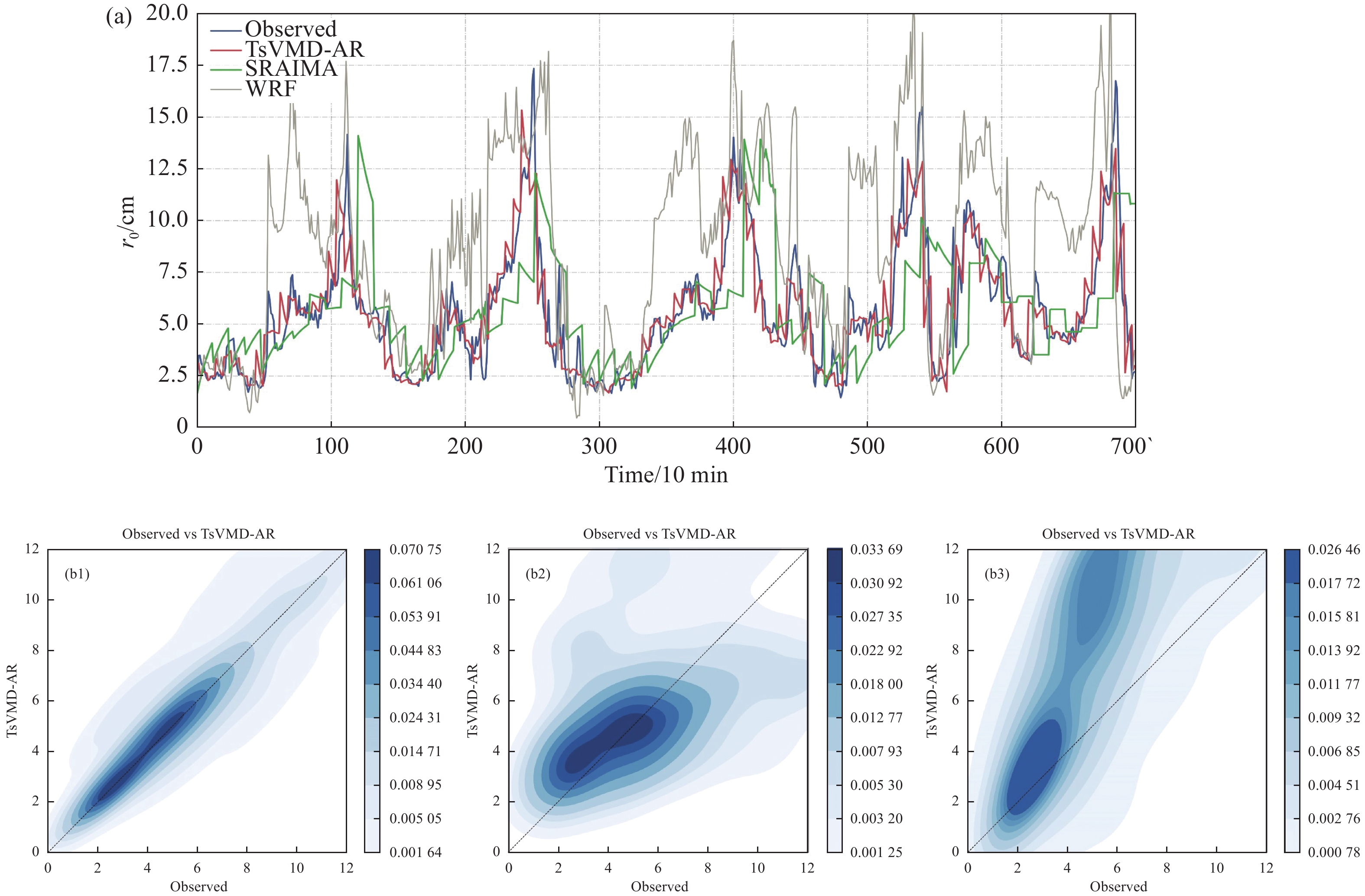
为了验证该模型的预测性能,采用遥感卫星地面站观测数据集对WRF和季节性自回归综合移动平均 (SARIMA)进行了比较。如图6 所示,TsVMD-AR模型更符合观测值的趋势,其预测精度明显更高,特别是对于突变。观测值和预测值散点图的二维直方图如图6(b)~(d) 所示。可以看出,TsVMD-AR模型可以得到最均匀、最接近的回归线分布。

图 6 TSVMD-AR模式和其他方法的湍流预报结果对比结果[98]。(a)实测湍流(蓝色)和TsVMD-AR(红色)、SARIMA(绿色)和WRF(灰色)预报结果;(b)~(d)观测到的大气湍流二维直方图与TsVMD-AR(b)、SARIMA(c)和WRF(d)的预报结果对比
Figure 6. Turbulence forecasting results of the TsVMD-AR model and the other schemes[98]. (a) Observed atmospheric turbulence results (blue), and forecasting results through TsVMD-AR (red), SARIMA (green) and WRF (grey); (b)-(d) 2D histograms of observed atmospheric turbulence result verse forecasting results of TsVMD-AR(b), SARIMA(c) and WRF(d)
TsVMD-AR、SARIMA和WRF模型预报的定量结果如图7 所示,结果表明,与WRF模型相比,TsVMD-AR模型和SARIMA模型的RMSE、MAPE和MAE分别降低了74.5%、80.2%、78.5%和49.4%、53.9%、52.4%。

TsVMD-AR与SARIMA相比也具有一定的优势。与SARIMA模型相比,TsVMD-AR模型的RMSE、MAPE和MAE分别降低了48.4%、53.2%和52.7%。这可能是因为对数据集进行VMD分解后的imf更加稳定,相对更有规则性,减少了数据集中多尺度特征信息之间的干扰和耦合,使得数据集复杂的内部特征(包括线性和非线性特征)更容易获得,降低了预测模型的难度。同时,方法利用VMD提取数据集中的低至高频信息,能较好地捕捉和预测大气湍流的突变。因此,与SARIMA模型相比,该方法具有更好的峰谷预测精度。值得一提的是,TsVMD-AR模型主要针对未来2 h的短时预报场景,由于实测大气相干长度数据在2 h内的自相关性更好,并且大气条件具有复杂性和多变性,以及长期预测中可能遇到的不确定性增加问题。长期预测需要考虑更多的变量和潜在的气候变化因素来选择合适的模型。
TsVMD-AR、SARIMA和WRF模型预报的定性和定量结果表明,TsVMD-AR模型优于其他模型,适合日常大气湍流预报。这种高精度的大气湍流预报为星地光数据传输链路的自适应波前补偿提供了一种策略,有望显著提高数据传输可靠性。
-
文中主要综述了面向星地激光通信的大气光学湍流预报的国内外研究进展。主要介绍了中尺度数值预报方法、基于深度学习的预报方法等。中尺度数值预报方法较为成熟且应用广泛,但存在分辨率有限、湍流参数化方案准确性不足等问题。基于深度学习的预报方法具有较好的泛化能力,能够从复杂的数据中挖掘气象参数与$ {C}_{n}^{2} $的关系,但也存在预报准确性对气象参数预报的准确性要求较高的问题。最近,基于TsVMD-AR模型预报大气相干长度的方法为提升短时预报准确性和分辨率提出了一种新的方法,但仍需要在更多站址实际应用后不断优化和完善。随着计算机算力的提升以及气象预报准确性的提高,面向星地激光通信的大气光学湍流预报方案有望进一步在实际场景中应用。
Atmospheric optical turbulence prediction method for satellite-ground laser communication (invited)
-
摘要: 激光通信系统在大气环境下应用的性能受到严重制约,当激光在大气湍流中传输时,其波面会发生畸变。在激光通信系统中,对大气湍流相关参数进行预报可以提前对星地数据传输链路进行调度,避免建立无效的通信任务。此外,大气湍流预报在天文选址、光学遥感等领域也有重要价值。随着国内外相关工作的长期积累以及算力、观测设备等硬件的能力提升,当前科研人员已经提出了一些大气湍流预报方案。文中主要综述了国内外学者在大气湍流预报方面的研究进展,首先详细介绍了目前应用比较广泛的中尺度数值预报技术,列举了使用中尺度数值预报方法对国内外典型区域的大气湍流进行预报的相关工作;然后介绍了深度学习方法在大气湍流预报中的应用情况,对其优势与局限性进行了讨论;最后介绍了一种面向星地激光通信的大气相干长度短时预报方法。
-
关键词:
- 大气湍流 /
- 湍流预报 /
- $ {C}_{n}^{2} $廓线 /
- 大气相干长度
Abstract:Significance The prediction of atmospheric turbulence has great significance both in science and engineering, which provides key parameters and references for domains like astronomical observation, site selection, satellite-ground laser communication, and remote sensing. Especially in satellite-ground laser communication, predicting key parameters of atmospheric turbulence can schedule satellite-ground data transmission links in advance, and pre-deploy adaptive optical schemes to compensate turbulence effects, so as to establish effective communication links and suppress the performance degradation of data transmission. Therefore, atmospheric turbulence prediction is crucial and become an important issue, which needs to be addressed for most of laser scenarios in atmosphere. Progress This review consists of three sections. In the first section, firstly, the widely used meso-scale numerical prediction scheme to forecast atmospheric turbulence is introduced in detail. This scheme is accomplished by turbulence parameterization schemes, which establishes the relationship between the turbulence characteristics and the conventional meteorological parameters output from mesoscale meteorological model. Mesoscale meteorological model has been well developed, the most representative models include Meso-Nh(Non-hydrostatic mesoscale atmospheric model), MM5(Mesoscale Model 5), WRF(Weather Research & Forecasting Model) and Polar WRF. Many achievements have been made in turbulence parameterization schemes, including Hufmagel model, Tatarski model. Then, the relevant work of using mesoscale numerical prediction method to forecast atmospheric turbulence in typical regions is reviewed. The second section presents recent advances regarding deep learning in atmospheric turbulence prediction, and discusses its advantages and limitations. This section first introduces the research achievements of deep learning in meteorological forecasting, and then introduces the research advances of deep learning in atmospheric turbulence forecasting. Based on a large amount of data, deep learning scheme can establish a relationship between the input data and the target label without any prior formula. In atmospheric turbulence prediction, deep learning is used to establish the relationship between meteorological parameters and atmospheric turbulence parameters, but the prediction accuracy is also limited by the accuracy of meteorological parameters. In the third section, a short-time atmospheric coherence length prediction method called TsVMD-AR is introduced. TsVMD-AR model uses VMD (variational mode decomposition) algorithm and AR (autoregression) algorithm to forecast the short-term atmospheric coherence length. This scheme reduces the interference and coupling between the multi-scale feature information in the dataset, makes the complex internal features of the dataset easier to obtain. The results show that the established TsVMD-AR model is obviously superior to other models and is suitable for daily atmospheric turbulence prediction. Prospects We hope this review will provide more valuable information for people who is working in scenarios of laser applications in atmosphere turbulence, and inspire more wonderful ideas towards abilities of more accurate and faster turbulence grasp. -
图 1 大气湍流的中尺度数值预报。(a) Cerro Paranal台址模型计算结果与实测$ {C}_{n}^{2} $廓线的对比[33];(b) WRF预报系统工作流程图[25];(c) 高美古WRF预报结果与实测结果的比较
Figure 1. The meso-scale numerical prediction of atmosphere turbulence. (a) Results comparison between the model of Cerro Paranal station site and the measured $ {C}_{n}^{2} $ profiles[33]; (b) WRF modeling system flow chart[25]; (c) Comparison of WRF and measured data at Gaomeigu
图 4 基于深度学习的大气光学湍流预报方案。(a) BP算法网络结构[87];(b) AGA-BP 神经网络结构[89];(c)实测值、AGA-BP 网络预报值、Polar WRF预报值的比对结果[89]
Figure 4. Atmospheric optical turbulence prediction through deep learning. (a) BP neural network[87]; (b) AGA-BP neural network[89]; (c) Results of measured data, Polar WRF prediction, AGA-BP neural network prediction[89]
图 6 TSVMD-AR模式和其他方法的湍流预报结果对比结果[98]。(a)实测湍流(蓝色)和TsVMD-AR(红色)、SARIMA(绿色)和WRF(灰色)预报结果;(b)~(d)观测到的大气湍流二维直方图与TsVMD-AR(b)、SARIMA(c)和WRF(d)的预报结果对比
Figure 6. Turbulence forecasting results of the TsVMD-AR model and the other schemes[98]. (a) Observed atmospheric turbulence results (blue), and forecasting results through TsVMD-AR (red), SARIMA (green) and WRF (grey); (b)-(d) 2D histograms of observed atmospheric turbulence result verse forecasting results of TsVMD-AR(b), SARIMA(c) and WRF(d)
-
[1] Chen M, Liu C, Rui D, et al. Performance verification of adaptive optics for satellite-to-ground coherent optical communications at large zenith angle [J]. Optics Express, 2018, 26(4): 4230-4242. doi: 10.1364/OE.26.004230 [2] Hemmati H, Biswas A, Djordjevic I B. Deep-space optical communications: Future perspectives and applications [J]. Proceedings of the IEEE, 2011, 99(11): 2020-2039. doi: 10.1109/JPROC.2011.2160609 [3] Oaida B V, Wu W, Erkmen B I, et al. Optical link design and validation testing of the Optical Payload for Lasercomm Science (OPALS) system[C]//Free-Space Laser Communication and Atmospheric Propagation XXVI. SPIE, 2014, 8971: 235-249. [4] Smutny B, Kaempfner H, Muehlnikel G, et al. 5.6 Gbps optical intersatellite communication link[C]//Free-Space Laser Communication Technologies XXI, SPIE, 2009, 7199: 38-45. [5] Fu S, Zhai Y, Zhou H, et al. Experimental demonstration of free-space multi-state orbital angular momentum shift keying [J]. Optics Express, 2019, 27(23): 33111-33119. doi: 10.1364/OE.27.033111 [6] Fu S, Zhai Y, Zhou H, et al. Demonstration of free-space one-to-many multicasting link from orbital angular momentum encoding [J]. Optics Letters, 2019, 44(19): 4753-4756. doi: 10.1364/OL.44.004753 [7] Krenn M, Handsteiner J, Fink M, et al. Twisted light transmission over 143 km [J]. Proceedings of the National Academy of Sciences, 2016, 113(48): 13648-13653. doi: 10.1073/pnas.1612023113 [8] Wang J, Yang J Y, Fazal I M, et al. Terabit free-space data transmission employing orbital angular momentum multiplexing [J]. Nature Photonics, 2012, 6(7): 488-496. doi: 10.1038/nphoton.2012.138 [9] Jahid A, Alsharif M H, Hall T J. A contemporary survey on free space optical communication: Potentials, technical challenges, recent advances and research direction [J]. Journal of Network and Computer Applications, 2022, 200: 103311. doi: 10.1016/j.jnca.2021.103311 [10] Sadiku M N O, Musa S M, Nelatury S R. Free space optical communications: An overview [J]. European Scientific Journal, 2016, 12(9): 55-68. doi: 10.19044/esj.2016.v12n9p55 [11] Zhu Z, Janasik M, Fyffe A, et al. Compensation-free high-dimensional free-space optical communication using turbulence-resilient vector beams [J]. Nature Communications, 2021, 12(1): 1666. doi: 10.1038/s41467-021-21793-1 [12] Good R E, Beland R R, Murphy E A, et al. Atmospheric models of optical turbulence[C]//Modeling of the Atmosphere, SPIE, 1988, 928: 165-186. [13] Ata Y, Baykal Y, Gökçe M C. Average channel capacity in anisotropic atmospheric non-Kolmogorov turbulent medium [J]. Optics Communications, 2019, 451: 129-135. doi: 10.1016/j.optcom.2019.06.055 [14] Baykal Y, Gerçekcioğlu H. Multimode laser beam scintillations in strong atmospheric turbulence [J]. Applied Physics B, 2019, 125(8): 152. doi: 10.1007/s00340-019-7269-x [15] Chiba T. Spot dancing of the laser beam propagated through the turbulent atmosphere [J]. Applied Optics, 1971, 10(11): 2456-2461. doi: 10.1364/AO.10.002456 [16] Li M, Li B, Zhang X, et al. Investigation of the phase fluctuation effect on the BER performance of DPSK space downlink optical communication system on fluctuation channel [J]. Optics Communications, 2016, 366: 248-252. doi: 10.1016/j.optcom.2016.01.003 [17] Yang Q, Li L, Guo P, et al. Effects of atmospheric turbulence on fiber-coupled DPSK system in satellite-to-ground downlink [J]. Results in Physics, 2018, 11: 938-943. doi: 10.1016/j.rinp.2018.10.056 [18] Kang H J, Yang J, Chun B J, et al. Free-space transfer of comb-rooted optical frequencies over an 18 km open-air link [J]. Nature Communications, 2019, 10(1): 4438. doi: 10.1038/s41467-019-12443-8 [19] Fu S, Gao C. Influences of atmospheric turbulence effects on the orbital angular momentum spectra of vortex beams [J]. Photonics Research, 2016, 4(5): B1-B4. doi: 10.1364/PRJ.4.0000B1 [20] Baykal Y. Scintillation index in strong oceanic turbulence [J]. Optics Communications, 2016, 375: 15-18. doi: 10.1016/j.optcom.2016.05.002 [21] Wang Y, Xu H, Li D, et al. Performance analysis of an adaptive optics system for free-space optics communication through atmospheric turbulence [J]. Scientific Reports, 2018, 8(1): 1124. doi: 10.1038/s41598-018-19559-9 [22] Liu C, Chen S, Li X Y, et al. Performance evaluation of adaptive optics for atmospheric coherent laser communications [J]. Optics Express, 2014, 22(13): 15554-15563. doi: 10.1364/OE.22.015554 [23] Yang L, Yao K, Wang J, et al. Performance analysis of 349-element adaptive optics unit for a coherent free space optical communication system [J]. Scientific Reports, 2019, 9(1): 13150. doi: 10.1038/s41598-019-48338-3 [24] Hufnagel R E, Stanley N R. Modulation transfer function associated with image transmission through turbulent media [J]. JOSA, 1964, 54(1): 52-61. doi: 10.1364/JOSA.54.000052 [25] Jiménez P A, Dudhia J, González-Rouco J F, et al. A revised scheme for the WRF surface layer formulation [J]. Monthly Weather Review, 2012, 140(3): 898-918. doi: 10.1175/MWR-D-11-00056.1 [26] Tapp M C, White P W. A non‐hydrostatic mesoscale model [J]. Quarterly Journal of the Royal Meteorological Society, 1976, 102(432): 277-296. doi: 10.1002/qj.49710243202 [27] Chen F, Dudhia J. Coupling an advanced land surface–hydrology model with the Penn State–NCAR MM5 modeling system. Part I: Model implementation and sensitivity [J]. Monthly Weather Review, 2001, 129(4): 569-585. [28] Tatarski V I. Wave Propagation in a Turbulent Medium[M]. Courier Dover Publications, 2016. [29] Dewan E M. A Model for C2n (optical turbulence) profiles using radiosonde data[M]// Directorate of Geophysics, Air Force Materiel Command, 1993. [30] Coulman C E, Vernin J. Significance of anisotropy and the outer scale of turbulence for optical and radio seeing [J]. Applied Optics, 1991, 30(1): 118-126. doi: 10.1364/AO.30.000118 [31] Ruggiero F H, DeBenedictis D A. Forecasting optical turbulence from mesoscale numerical weather prediction models[C]//DoD High Performance Modernization Program Users Group Conference, 2002: 10-14. [32] Coulman C E, Andre J C, Lacarrere P, et al. The observation, calculation, and possible forecasting of astronomical seeing [J]. Publications of the Astronomical Society of the Pacific, 1986, 98(601): 376. [33] Masciadri E, Vernin J, Bougeault P. 3D mapping of optical turbulence using an atmospheric numerical model-I. a useful tool for the ground-based astronomy [J]. Astronomy and Astrophysics Supplement Series, 1999, 137(1): 185-202. doi: 10.1051/aas:1999474 [34] Masciadri E, Vernin J, Bougeault P. 3D mapping of optical turbulence using an atmospheric numerical model. II. first results at Cerro Paranal [J]. Astronomy and Astrophysics Supplement Series, 1999, 137: 203-216. doi: 10.1051/aas:1999475 [35] Cheinet S, Beljaars A, Weiss-Wrana K, et al. The use of weather forecasts to characterise near-surface optical turbulence [J]. Boundary-Layer Meteorology, 2011, 138(3): 453-473. doi: 10.1007/s10546-010-9567-z [36] Cherubini T, Businger S, Lyman R, et al. Modeling optical turbulence and seeing over Mauna Kea [J]. Journal of Applied Meteorology and Climatology, 2008, 47(4): 1140-1155. doi: 10.1175/2007JAMC1487.1 [37] Masciadri E. Optical turbulence forecast: toward a new era of ground-based astronomy[C]//Ground-based and Airborne Telescopes, SPIE, 2006, 6267: 461-468. [38] Cherubini T, Businger S, Lyman R. Modeling optical turbulence and seeing over Mauna Kea: Verification and algorithm refinement [J]. Journal of Applied Meteorology and Climatology, 2008, 47(12): 3033-3043. doi: 10.1175/2008JAMC1839.1 [39] Mahalov A, Moustaoui M. Characterization of atmospheric optical turbulence for laser propagation [J]. Laser & Photonics Reviews, 2010, 4(1): 144-159. [40] Lascaux F, Masciadri E, Fini L. MOSE: Operational forecast of the optical turbulence and atmospheric parameters at European Southern Observatory ground-based sites–II. Atmospheric parameters in the surface layer 0–30 m [J]. Monthly Notices of the Royal Astronomical Society, 2013, 436(4): 3147-3166. doi: 10.1093/mnras/stt1803 [41] Wu X, Zeng Z, Xiao Li, et al. Observations of atmospheric turbulence by balloon-borne instrument at Xinlong station [J]. Chinese Journal of Quantum Electronics, 1996, 13(4): 385-390. (in Chinese) [42] Weng N, Zeng Z, Xiao L, et al. Profile and characteristic of refractive index structure constant [J]. High Power Laser and Particle Beams, 1999, 11(6): 673-676. (in Chinese) [43] Wu X, Sun G, Weng N, et al. Measurement and modeling of $ {C}_{n}^{2} $ at typical regions in China [J]. Journal of Atmospheric and Environmental Optics, 2007, 2(6): 409-422. (in Chinese) [44] Sun G, Weng N, Xiao L. Vertical distribution models of atmospheric structure constant of refractive index [J]. High Power Laser and Particle Beams, 2008, 20(2): 183-188. (in Chinese) [45] Xu L, Wu X, Wang Y. Forecast optical turbulence with mesoscale weather forecast model [J]. Journal of Atmospheric and Environmental Optics, 2008(4): 270-275. (in Chinese) [46] Qing C, Wu X, Li X, et al. Estimation of atmospheric optical turbulence profile by WRF model at gaomeigu [J]. Chinese Journal of Lasers, 2015, 42(9): 316-323. (in Chinese) [47] Qing C, Wu X, Li X, et al. Research on simulating atmospheric optical turbulence in typical area [J]. Acta Optica Sinica, 2016, 36(5): 9-15. (in Chinese) [48] Qing C, Wu X, Li X, et al. Use of weather research and forecasting model outputs to obtain near-surface refractive index structure constant over the ocean [J]. Optics Express, 2016, 24(12): 13303-13315. doi: 10.1364/OE.24.013303 [49] Qing C, Wu X, Huang H, et al. Estimating the surface layer refractive index structure constant over snow and sea ice using Monin-Obukhov similarity theory with a mesoscale atmospheric model [J]. Optics Express, 2016, 24(18): 20424-20436. doi: 10.1364/OE.24.020424 [50] Qing C, Bi C, Zhu W, et al. A global turbulence model shows excellent atmospheric optical turbulence conditions over the Ethiopian plateau during non-rainy season [J]. Monthly Notices of the Royal Astronomical Society, 2023, 526(1): 802-807. doi: 10.1093/mnras/stad2795 [51] Wang H, Yao Y, Liu L. A review of atmospheric optical turbulence modeling research [J]. Progress in Astronomy, 2012, 30(3): 362-377. (in Chinese) [52] Wang H, Yao Y, Qian X, et al. The method of modeling atmospheric optical turbulence [J]. Acta Astronomica Sinica, 2012, 53(6): 527-537. (in Chinese) [53] Wang H, Yao Y, Liu L. Forecast of atmosphere optical turbulence at ali site by weather research and forecasting model [J]. Acta Optica Sinica, 2013, 33(3): 46-50. (in Chinese) [54] Qian X, Yao Y, Zou L, et al. Modelling of atmospheric optical turbulence with the weather research and forecasting model at the ali observatory, tibet [J]. Monthly Notices of the Royal Astronomical Society, 2021, 505(1): 582-592. doi: 10.1093/mnras/stab1316 [55] LeCun Y, Bengio Y, Hinton G. Deep learning [J]. Nature, 2015, 521(7553): 436-444. doi: 10.1038/nature14539 [56] Badrinarayanan V, Kendall A, Cipolla R. SegNet: A deep convolutional encoder-decoder architecture for image segmentation [J]. IEEE Transactions on Pattern Analysis and Machine Intelligence, 2017, 39(12): 2481-2495. doi: 10.1109/TPAMI.2016.2644615 [57] Ronneberger O, Fischer P, Brox T. U-net: Convolutional networks for biomedical image segmentation[C]//Medical Image Computing and Computer-Assisted Intervention–MICCAI 2015: 18th International Conference, Munich, Germany, October 5-9, 2015, Proceedings, Part III 18. Springer International Publishing, 2015: 234-241. [58] Roy A G, Conjeti S, Karri S P K, et al. ReLayNet: Retinal layer and fluid segmentation of macular optical coherence tomography using fully convolutional networks [J]. Biomedical Optics Express, 2017, 8(8): 3627-3642. doi: 10.1364/BOE.8.003627 [59] Chen H, Zhang Y, Zhang W, et al. Low-dose CT via convolutional neural network [J]. Biomedical Optics Express, 2017, 8(2): 679-694. doi: 10.1364/BOE.8.000679 [60] Fang L, Cunefare D, Wang C, et al. Automatic segmentation of nine retinal layer boundaries in OCT images of non-exudative AMD patients using deep learning and graph search [J]. Biomedical Optics Express, 2017, 8(5): 2732-2744. doi: 10.1364/BOE.8.002732 [61] Lee C S, Tyring A J, Deruyter N P, et al. Deep-learning based, automated segmentation of macular edema in optical coherence tomography [J]. Biomedical Optics Express, 2017, 8(7): 3440-3448. doi: 10.1364/BOE.8.003440 [62] Mnih V, Kavukcuoglu K, Silver D, et al. Human-level control through deep reinforcement learning [J]. Nature, 2015, 518(7540): 529-533. doi: 10.1038/nature14236 [63] Wang K, Dou J, Kemao Q, et al. Y-Net: a one-to-two deep learning framework for digital holographic reconstruction [J]. Optics Letters, 2019, 44(19): 4765-4768. doi: 10.1364/OL.44.004765 [64] Rivenson Y, Zhang Y, Günaydın H, et al. Phase recovery and holographic image reconstruction using deep learning in neural networks [J]. Light:Science & Applications, 2018, 7(2): 17141-17141. [65] Wu Y, Rivenson Y, Zhang Y, et al. Extended depth-of-field in holographic imaging using deep-learning-based autofocusing and phase recovery [J]. Optica, 2018, 5(6): 704-710. doi: 10.1364/OPTICA.5.000704 [66] Wang K, Li Y, Kemao Q, et al. One-step robust deep learning phase unwrapping [J]. Optics Express, 2019, 27(10): 15100-15115. doi: 10.1364/OE.27.015100 [67] Barbastathis G, Ozcan A, Situ G. On the use of deep learning for computational imaging [J]. Optica, 2019, 6(8): 921-943. doi: 10.1364/OPTICA.6.000921 [68] Rahmani B, Loterie D, Konstantinou G, et al. Multimode optical fiber transmission with a deep learning network [J]. Light: Science & Applications, 2018, 7(1): 69. [69] Sinha A, Lee J, Li S, et al. Lensless computational imaging through deep learning [J]. Optica, 2017, 4(9): 1117-1125. doi: 10.1364/OPTICA.4.001117 [70] Borhani N, Kakkava E, Moser C, et al. Learning to see through multimode fibers [J]. Optica, 2018, 5(8): 960-966. doi: 10.1364/OPTICA.5.000960 [71] Wang F, Wang H, Wang H, et al. Learning from simulation: An end-to-end deep-learning approach for computational ghost imaging [J]. Optics Express, 2019, 27(18): 25560-25572. doi: 10.1364/OE.27.025560 [72] Li S, Deng M, Lee J, et al. Imaging through glass diffusers using densely connected convolutional networks [J]. Optica, 2018, 5(7): 803-813. doi: 10.1364/OPTICA.5.000803 [73] Li Y, Xue Y, Tian L. Deep speckle correlation: a deep learning approach toward scalable imaging through scattering media [J]. Optica, 2018, 5(10): 1181-1190. doi: 10.1364/OPTICA.5.001181 [74] Nguyen T, Xue Y, Li Y, et al. Deep learning approach for Fourier ptychography microscopy [J]. Optics Express, 2018, 26(20): 26470-26484. doi: 10.1364/OE.26.026470 [75] Dong C, Loy C C, He K, et al. Image super-resolution using deep convolutional networks [J]. IEEE Transactions on Pattern Analysis and Machine Intelligence, 2015, 38(2): 295-307. [76] Nehme E, Weiss L E, Michaeli T, et al. Deep-STORM: super-resolution single-molecule microscopy by deep learning [J]. Optica, 2018, 5(4): 458-464. doi: 10.1364/OPTICA.5.000458 [77] Rivenson Y, Göröcs Z, Günaydin H, et al. Deep learning microscopy [J]. Optica, 2017, 4(11): 1437-1443. doi: 10.1364/OPTICA.4.001437 [78] Huang T, Zhang Q, Liu J, et al. Adversarial attacks on deep-learning-based SAR image target recognition [J]. Journal of Network and Computer Applications, 2020, 162: 102632. doi: 10.1016/j.jnca.2020.102632 [79] Wang D, Zhang M, Li J, et al. Intelligent constellation diagram analyzer using convolutional neural network-based deep learning [J]. Optics Express, 2017, 25(15): 17150-17166. doi: 10.1364/OE.25.017150 [80] He K, Zhang X, Ren S, et al. Deep residual learning for image recognition[C]//Proceedings of the IEEE Conference on Computer Vision and Pattern Recognition, 2016: 770-778. [81] French M N, Krajewski W F, Cuykendall R R. Rainfall forecasting in space and time using a neural network [J]. Journal of Hydrology, 1992, 137(1-4): 1-31. doi: 10.1016/0022-1694(92)90046-X [82] Liu J N K, Kwong K M, Chan P W. Chaotic oscillatory-based neural network for wind shear and turbulence forecast with LiDAR data [J]. IEEE Transactions on Systems, Man, and Cybernetics, Part C (Applications and Reviews), 2012, 42(6): 1412-1423. doi: 10.1109/TSMCC.2012.2188284 [83] Qiu M, Zhao P, Zhang K, et al. A short-term rainfall prediction model using multi-task convolutional neural networks[C]//2017 IEEE International Conference on Data Mining (ICDM), IEEE, 2017: 395-404. [84] Sun Q, Jiao R, Xia J, et al. Adjusting wind speed prediction of numerical weather forecast model based on machine learning methods [J]. Meteor Mon, 2019, 45(3): 426-436. (in Chinese) [85] Sønderby C K, Espeholt L, Heek J, et al. Metnet: A neural weather model for precipitation forecasting [DB/OL]. (2020-03-24). [2024-01-10].https://doi.org/10.48550/arXiv.2003.12140 [86] Andrychowicz M, Espeholt L, Li D, et al. Deep learning for day forecasts from sparse observations [DB/OL]. (2023-06-06). [2024-01-10].https://doi.org/10.48550/arXiv.2306.06079 [87] Wang Y, Basu S. Using an artificial neural network approach to estimate surface-layer optical turbulence at Mauna Loa, Hawaii [J]. Optics Letters, 2016, 41(10): 2334-2337. doi: 10.1364/OL.41.002334 [88] Lü J, Zhu W, Cai J, et al. Comparison of two approaches for estimating atmospheric optical turbulence intensity near sea [J]. Acta Optica Sinica, 2017, 37(5): 9-17. (in Chinese) [89] Su C, Wu X, Luo T, et al. Adaptive niche-genetic algorithm based on backpropagation neural network for atmospheric turbulence forecasting [J]. Applied Optics, 2020, 59(12): 3699-3705. doi: 10.1364/AO.388959 [90] Mahalov A, Moustaoui M, Grubišić V. A numerical study of mountain waves in the upper troposphere and lower stratosphere [J]. Atmospheric Chemistry and Physics, 2011, 11(11): 5123-5139. doi: 10.5194/acp-11-5123-2011 [91] DuVivier A K, Cassano J J. Evaluation of WRF model resolution on simulated mesoscale winds and surface fluxes near Greenland [J]. Monthly Weather Review, 2013, 141(3): 941-963. doi: 10.1175/MWR-D-12-00091.1 [92] Iriza A, Dumitrache R C, Lupascu A, et al. Studies regarding the quality of numerical weather forecasts of the WRF model integrated at high-resolutions for the Romanian territory [J]. Atmósfera, 2016, 29(1): 11-21. [93] Liu L Y, Giordano C, Yao Y Q, et al. Optical turbulence characterization at LAMOST site: Observations and models [J]. Monthly Notices of the Royal Astronomical Society, 2015, 451(3): 3299-3308. doi: 10.1093/mnras/stv1165 [94] Giordano C, Rafalimanana A, Ziad A, et al. Contribution of statistical site learning to improve optical turbulence forecasting [J]. Monthly Notices of the Royal Astronomical Society, 2021, 504(2): 1927-1938. doi: 10.1093/mnras/staa3709 [95] Basu S, He P. Quantifying the dependence of temperature and refractive index structure parameters on atmospheric stability using direct and large-eddy simulations[C]//Propagation Through and Characterization of Distributed Volume Turbulence, Optica Publishing Group, 2014: PM2E. 3. [96] Abahamid A, Vernin J, Benkhaldoun Z, et al. Seeing, outer scale of optical turbulence, and coherence outer scale at different astronomical sites using instruments on meteorological balloons [J]. Astronomy & Astrophysics, 2004, 422(3): 1123-1127. [97] Jellen C, Oakley M, Nelson C, et al. Machine-learning informed macro-meteorological models for the near-maritime environment [J]. Applied Optics, 2021, 60(11): 2938-2951. doi: 10.1364/AO.416680 [98] Li Y, Li L, Guo Y, et al. Atmospheric turbulence forecasting using two-stage variational mode decomposition and autoregression towards free-space optical data-transmission link [J]. Frontiers in Physics, 2022, 10: 970025. doi: 10.3389/fphy.2022.970025 [99] Dragomiretskiy K, Zosso D. Variational mode decomposition [J]. IEEE Transactions on Signal Processing, 2013, 62(3): 531-544. [100] He Y, Sheng Z, Zhu Y, et al. Adaptive variational mode decomposition method for eliminating instrument noise in turbulence detection [J]. Journal of Atmospheric and Oceanic Technology, 2021, 38(1): 31-46. doi: 10.1175/JTECH-D-20-0004.1 [101] Poggi P, Muselli M, Notton G, et al. Forecasting and simulating wind speed in Corsica by using an autoregressive model [J]. Energy Conversion and Management, 2003, 44(20): 3177-3196. doi: 10.1016/S0196-8904(03)00108-0 -

 点击查看大图

计量
- 文章访问数: 89
- HTML全文浏览量: 8
- PDF下载量: 47
- 被引次数: 0

