Multi-camera fast bundle adjustment algorithm based on normalized matrix dimensionality reduction

视觉测量技术是精密测量技术领域内最具有发展潜力的新技术。由于具有非接触、速度快、精度高、柔性好等诸多优点，视觉测量技术被广泛运用在目标识别与定位、导航、目标质量检测等各个领域^[1~3]。

在高精度视觉测量中，利用影像进行定位的光束法平差(Bundle Adjustment, BA)整体优化算法一直以来备受学者关注。Lourakis等人出于对BA运算过程中雅可比矩阵与法化矩阵的稀疏特性的研究，实现了基于稀疏矩阵的光束法平差(Sparse Bundle Adjustment, SBA)，大幅提升了内存使用与运算的效率^[4]；Snavely等人利用SBA算法结合网络上大量的场景图片进行了一系列三维重建实验^[5]，能够较为方便地实现三角网格重构的再生成效果。Wu等人^[6]在保持算法收敛性能的同时，利用并行计算使得SBA的运算速率提升约30倍，但是得到的参数精度有待进一步提升。薛俊鹏等人^[7]抓住了双目视觉中相机间位姿固定的关系，在双目领域中优化了算法，使得速度与精度都得到了提升，但是对于多相机系统的关系构建以及位置分布并没有给出相应的策略。夏泽民等人^[8]在双目光束法平差的基础上，加入相机内参相等的约束条件，使得精度更高。但是这些算法只适用于双目视觉系统，如果直接应用到多相机系统，则会使法化矩阵的维度大幅升高，平差矩阵难以解算，导致最终的收敛效果较差甚至求解失败。

当前多相机系统具有视场大、覆盖区域完善的特点，可以极大的提升视觉定位与跟踪性能^[9]，从而在无人驾驶、光控工厂、视觉导航等领域得到广泛地应用^[10-12]。因此多相机成像、标定以及重建的精度也成为广泛聚焦并值得深入研究的问题^[13-14]。对于多相机系统内外参数获取的研究中，参考文献[15]中徐秋宇等人基于精密角度优化了多相机定位系统的标定，提高了相机内参的精度；而Chen等人^[16]则通过引入惩罚因子计算出多相机的外部参数并保证了算法的灵活性与鲁棒性。然而这些算法都是从相机标定的角度出发，并没有同时优化相机拍摄的三维点坐标，以此来提高参数获取的精度。

基于上述分析，文中引入光束法平差算法进行多相机系统参数的获取与优化，提出一种基于法化矩阵降维的多相机快速光束法平差算法。将多个相机捆绑为一个优化整体的同时，根据相机间的固定位姿关系设置主从相机。由于从相机的位姿可以由主相机表示，在每次迭代运算时只需要对主相机的位姿参数与三维点进行优化便可以得到所有相机与空间点的综合优化更新，通过完成对法化矩阵的有效降维，得到超定方程的可行解，同时提高了全局收敛求解的速度，因此在一次迭代过程中能够完成对多个相机特征图像的运算。最终文中方法实现了多相机捆绑对场景进行拍摄，使得待优化参数相对减少，进而导致算法执行效率较高且减小了参数误差。最后通过模拟实验与实测实验验证该算法的有效性与精确性。

光束法平差是对空间中每一个三维点坐标以及每一个相机外参的整体求解与综合校正。其数学模型就是构建光束法平差中观测数据与参数之间的关系。它首先包括成像模型，如图1所示，即图像、物体及相机之间的数学关系，三者通常满足共线方程。根据此可以推导出重投影误差方程。其次是运用迭代方法对此非线性方程进行求解。

Figure 1.  Camera imaging model

由图像上的二维像素坐标变换到空间中的三维坐标需要两步，即由相机坐标系变换到像素坐标系的内参矩阵和由相机坐标系变换到世界坐标系的外参矩阵。齐次化之后用公式表达如下：

式中：$(X,Y,Z)$为三维世界坐标；$(u,v)$为二维理想像素坐标；$\lambda $为非零尺度因子；${{K}}$为相机内参；$({{R}},{{T}})$为相机外参，分别为旋转矩阵和平移矩阵；$s$为倾斜因子，一般不考虑。

然而在实际应用中，所有相机都难免存在一定程度畸变，而前文建立的模型是理想的线性模型，并没有涉及相机的畸变。因此，文中引入畸变模型来更真实地反映实际成像效果，由于切向畸变可以忽略，因此只考虑相机的径向畸变并且通过级数展开保留前2项，即2个参数，则有：

式中：$(x,y)$为二维点在图像坐标系下的坐标；${k_1},{k_2}$为径向畸变系数；$({u_d},{v_d})$为图像畸变后的实际坐标。

因此，将解算出来的三维点通过公式（1）与公式（2）的变换便可以得到重投影的像素坐标。将此坐标与对应特征点原像素坐标作差便可以得出重投影误差。求取所有特征点的重投影误差的二阶范数，并将公式（3）作为待优化的目标函数，表达如下：

式中：$m$为特征点的个数；$n$为相机个数或是图片个数；${u_{ij}}$为特征点在图像上的实际坐标；${\hat u_{ij}}$为重投影坐标；${w_{ij}}$为二值函数，值0表示此点不在图片上，值1表示此点在图片上。

因此，光束法平差本质上是$\delta $取得最小值时，相机外参以及空间坐标点的最优解的求取。

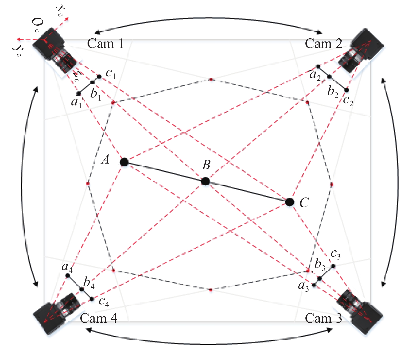
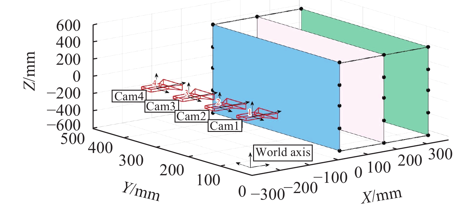
某些场合如卫星位置跟踪，为了保证精确性与实时性，不得不用多个相机同时进行拍摄。通常，在有多个相机对目标物体进行拍摄时，首先要对相机进行标定。可以通过张正友标定法进行相机标定，获取相机内外参数的初值。文中的策略是建立如图2所示的相机采集架构，全方位实现目标图像采集，将所有相机捆绑为一个整体。将其中一个相机作为主相机，将主相机的外参数作为光束法平差中待优化的参数。其他相机作为从相机，其相机外参可由主相机的外参经过变换求得。

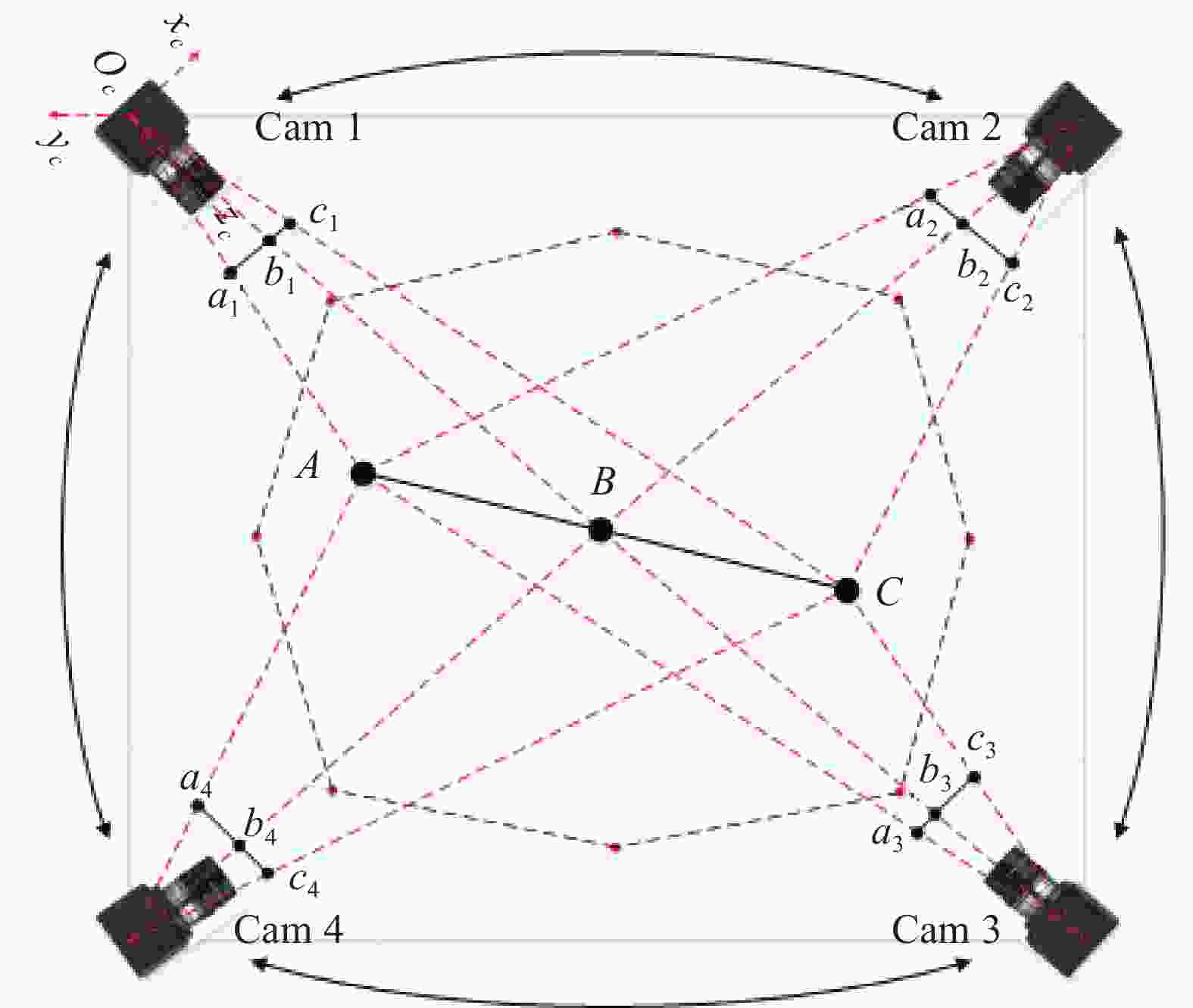
Figure 2.  Bundle adjustment structure of multi-camera system

假设有$k + 1$个相机，其中1个主相机，$k$个从相机，因此，根据传统的光束法平差，可以得出主相机的共线方程为：

式中：$({u_m},{v_m})$为主相机拍摄图片的像素坐标；${{{K}}_{{m}}}$为主相机的内参；$({{{R}}_{{m}}},{{{T}}_{{m}}})$为主相机的外参，即旋转矩阵和平移向量；$(X,Y,Z)$为三维点的世界坐标。

由共线方程对相机外参和三维点求一阶偏导可得误差方程如下：

式中：$({{{A}}_{{m}}},{{{B}}_{{m}}})$为${({u_m},{v_m})^{\rm T}}$对相机外参$({\omega _m},{\varphi _m},{\kappa _m},{t_{xm}}, $$ {t_{ym}},{t_{zm}})$和三维点$(X,Y,Z)$的一阶偏导数。

而且${({{{\delta }}_{{{cm}}}},{{{\delta }}_{{{tm}}}})^{\rm T}}$为主相机的外参改正数与三维点改正数，即每次迭代的步长，其可以表示为：

${{{L}}_{{m}}}$为图像上点的实际坐标与用共线方程计算得到的重投影坐标的差值矩阵：

综上所述，便得到了主相机的所有信息，基于法化矩阵降维的多相机的光束法平差就是为了充分利用从相机与主相机之间的固定约束关系，并将其他相机的外参用主相机的外参来表示。此时有$k + 1$个相机，其中一个为主相机，$k$个从相机，通过对所有相机的标定，可以得到从相机与主相机之间的固定几何约束关系$({{{R}}_{{{m1}}}},{{{T}}_{{{m1}}}}),({{{R}}_{{{m2}}}},{{{T}}_{{{m2}}}}) \cdots ({{{R}}_{{{mk}}}},{{{T}}_{{{mk}}}})$，则从相机的外参数$({{{R}}_{{k}}},{{{T}}_{{k}}})$可表示为：

根据上式可以推导出系统位姿变换矩阵，利用其进行的位姿变换可简化为：

因此，根据此约束关系，可以得出第$k$个相机的共线方程为：

式中：$({u_k},{v_k})$为第$k$个相机拍摄图像中的点的二维像素坐标；${{{K}}_{{k}}}$为第$k$个相机的内参。由共线方程对相机外参和三维点求一阶偏导，对三维点求导方式不变，但是对每个从相机的外参数求导，相当于对主相机的外参数求导，因此第$k$个从相机的误差方程可表示如下：

其中，

由公式（12）可以看出，只需要对主相机外部参数进行求导并且只用计算主相机外参和三维点的改正数即可。这极大程度上减少了对所有相机都进行运算的时间与运算量，下面对法化矩阵进行推导。首先得到雅可比矩阵${{J}}$为：

故法化矩阵为：

运用Levenberg-Marquardt算法进行求解，则法化方程为：

式中：${{L}} = {[ {{{{L _m}}}}\;\;{{{{L_1}}}}\;{{{{L_2}}}}\; \cdots \;{{{{L_k}}}} ]^{\rm{T}}}$。

由上述推导可以看出，相比于传统的光束法平差算法，新的光束法平差算法在优化处理时，方程总个数不变，但是待优化的参数减少了。假设有$k + 1$个相机对$n$个三维中的点拍摄$m$次。则传统的算法便有$6(k + 1)m + 3n$个待优化量，因为每个相机每次拍摄便会引入6个未知数，每个三维点引入3个未知数。而新算法加入相机位姿关系后只有$ 6m + 3n +k$个待优化量，因为有了相机间的约束关系，消除了因相机数量引入的未知数。单从相机参数考虑，待优化量比原先少了约$k + 1$倍，即法化矩阵的维数减少了约$k + 1$倍。并且随着相机数量增多，此算法的收益更大。

文中在传统光束法平差的基础上，建立基于法化矩阵降维的多相机快速光束法平差算法。为了验证此算法的优越之处。在仿真实验部分取空间中30个特征点构成一个长方体作为测试的三维点集，此长方体的尺寸设定为300 mm×400 mm×500 mm。设置4个等距离且平行的相机对场景进行模拟采集，作为第一组结果。然后将4个相机捆绑，同时向远离场景的方向每次平移10 mm并再次采集一次，一共采集4次，共产生16幅模拟图像。图3所示为模拟测试的三维点图空间分布。

Figure 3.  3D point space diagram of cuboid

在模拟实验中，设置4个相机内参相等，均为${f_u} = {f_v} = 2500\ \rm pixel$，${u_0} = 640\ \rm pixel$，${v_0} = 512\ \rm pixel$，$s = 0$。将16幅模拟图像中加入干扰，即高斯噪声。向相机外参和三维点中均加入相对误差为0%~5%等间距的高斯白噪声作为光束法平差的初值，并分别求出对应的重投影误差。

下面进行新算法精度的验证。首先比较算法的重投影误差的平均值。使用Levenberg-Marquardt算法进行50次迭代，计算出迭代前与迭代后的重投影误差并取平均值，每次取不同相对误差的高斯噪声。为了避免偶然性，取定一种相对误差后重复10次并取均值。实验结果如图4所示。

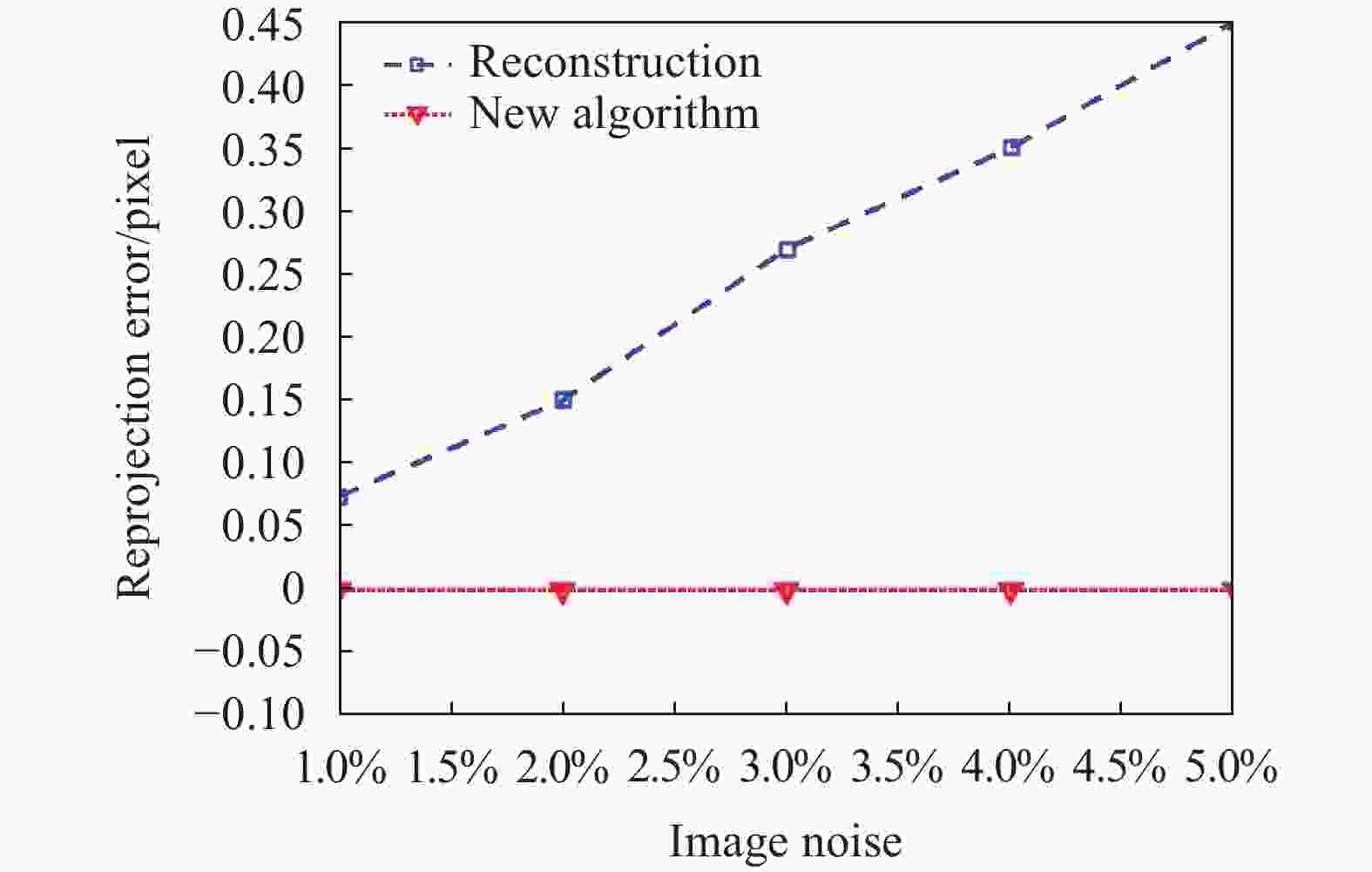
Figure 4.  Effect of Gaussian noise on reprojection error

由图4可以看出，随着噪声的增大，在新算法下图片的重投影误差并无明显的变化，说明此算法合理，并且可以达到预期的收敛效果。

然后，比较重建的三维点与真实三维点的误差。将重构点与真实点逐一求取距离，并取均值算出平均每一点的偏差量，相当于求解每一点的平均绝对误差。并与传统光束法平差算法进行比较，实验结果如图5所示。

Figure 5.  Effect of Gaussian noise on reconstructing 3D points

由图5可以看出，在不同的噪声下，新算法重建的三维点误差都要小于传统的算法结果，因此得到了优化。并且随着噪声的增大，优化的程度也更大，因为这里将4个相机捆绑为一个整体，相当于增加了传感器的数量，并且固定相机间的位姿关系，使得总体上方程个数增多，但未知数个数较传统算法而言却减少了。故新算法的重建精度较原来相比提升了约15.5%，重建精度得到了提升与优化。

为了进一步验证光束法平差新算法对优化相机参数与三维点的有效性，用4台Mikrotron相机MC3010进行拍摄。获取的图像尺寸为 $1\;680 \times 1\;710$ pixel，每个像素为0.008 mm/pixels，并且相机镜头型号均为AF Zoom-Nikkor 24-85 mm/1:2.8-4D。相机与靶标的捕获深度方向上距离约为3200 mm，相机采集系统架构如图6所示。

Figure 6.  Stereo camera system image acquisition equipment

通过图6中所示的4台相机对平面99圆靶标进行图像采集，采集到的图像分布如图7所示，并对每个标定板上的99特征点进行圆心提取与编号，图7中的编号值即为已经完成的特征点对应编码。

Figure 7.  Effect image of target image acquisition and center extraction

在图像采集完成之后，进行多相机系统的标定运算，由于型号相同，因此4个相机的内参在一定程度上相同，解算出相机的内参，以及从相机与主相机间的内外参关系如表1所示。

然后对99个圆心点的三维坐标与相机外参分别用传统的光束法平差和新算法进行优化处理，并将所有圆心点以空间三维分布进行显示，保留每个三维点的坐标值方便对比。重构出的靶板特征点空间三维布局效果图以及对应的编号如图8所示。

Figure 8.  3D points of the actual calibration plate

接着由表1得出的位姿关系，可以根据前文的推导计算出系统位姿变换矩阵的初值，如公式(16)所示。

将此矩阵作为相机外参之间的关系代入光束法平差算法中，将主相机的外参与99个三维点进行综合优化后得到的结果于真实值比较，并计算出每个点的误差以及所有点坐标的平均误差。表2给出其中连续11个编号点的坐标值以及平均误差值。

根据计算，得出用传统光束法平差时，最后得到的平均误差为每个点0.2946 mm，而新算法得到的误差为每个点0.1527 mm，再结合表2可以看出，文中算法可以得到很好的效果，并且对于多相机系统而言，新的算法在精度上更有优势。得到的三维点误差也更小，算法在重构精度及稳定性上均得到了优化。

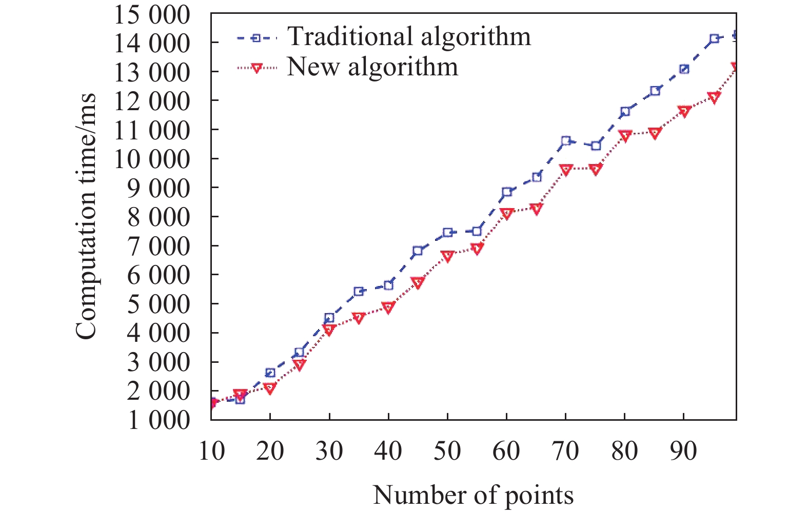
最后，为了验证新算法的效率优势，将新算法优化三维点的时间与原算法运行时间作比较，以点的个数作为自变量。观察重建点增加时两个算法的运行时间。实验结果如图9所示。

Figure 9.  Relationship between running time and number of 3D points

由图9可以看出，新算法在运行速率、执行效率上高于传统算法，这是因为将多个相机绑定为一个相机，那么在一次迭代过程中可以处理多幅图像，同时通过法化矩阵降维，实现运算速度的提升，并且随着三维点的增加，效果更加明显。根据运行时间与三维点数目关系计算得到新算法效率提升了约7.8%。

此算法优化处理多相机系统时，可以大幅度降低法化矩阵的维数，在精确性与快速性上占一定的优势。但是此算法在优化的过程中并没有对相机的内参进行优化。而在多相机系统领域，随着相机数量的增多，相机的内参也会对光束法平差结果产生一定的影响。因此后续在此算法的基础上，可以考虑在不改变算法效率的前提上，适当的加入相机内参从而在算法精度上完成进一步的提升，以适应于超大视场的高精度视觉测量与重构。

文中将稀疏光束法平差算法进行改进优化并引入到多相机系统中，充分利用每个相机间的固定位姿关系，将其中一个设置为主相机，其余的从相机外参用主相机关联表示，根据相机间特有的位姿关系，提出了系统变换矩阵，加入到光束法平差中进行快速变换，使得在光束法平差整体优化的过程中，待优化的参数相对减少，降低法化矩阵的维数，使优化结果精度与效率更高。最后通过仿真实验与实测实验验证了此算法的有效性与优越性。新算法在精度上提高了约15.5%，在效率上提高了约7.8%，得到的更为精确的结果能够满足如空间三维重构、自动停泊系统及医学图像定位等实际工程的应用需求。

下一步工作将基于多源数据融合，实现超大视场及高分遥感图像的立体重构与测量，通过冗余信息实现多相机系统内外参数统一全局优化。