


-
Infrared-visible image patches matching is a fundamental task of infrared-visible image processing. It compares the object or region by analyzing the similarity of content, features, structures, relationships, textures, and grayscales in infrared-visible images. The infrared-visible image matching is often used as a subroutine that plays an important role in a wide variety of applications, such as visual navigation[1-2] and target recognition[3-4].
Infrared-visible image patches is more challenging compared with traditional visible images. Since infrared and visible sensors use different imaging principles, the images taken by multiple sensors also have more differences than those by a single sensor. The edges of the object are blurred in infrared images. Less texture and color features are found in the object. The infrared-visible image pairs have significant grayscale distortion and illumination change.
Manual descriptors are used to extract features, such as SIFT[5], SURF[6], ORB[7], etc. The features extracted with the descriptors should have the invariance of illumination, rotation, scale, and affine. After feature extraction, image patches matching is predicted by comparison of features similarity. Most work is focused on improvements to infrared and visible image descriptors in the traditional infrared-visible image system. Sima[8] optimized the SIFT method for the infrared-visible image. Li[9] detected object edges and extracted the features of SURF to match the infrared-visible images. Chao Zhiguo[10] proposed a matching method based on histograms of oriented gradients used as the matching feature and the correlation coefficient used as a similar measure. Cao Zhiguo[11] adopted an approach to shape contexts for matching infrared-visible images based on their similar shape. Jiao Anbo[12] proposed the image matching algorithm using linear group geometric primitives for infrared and visible template matching.
Hand-craft descriptors need to improve continuously for new applications to extract efficient features. The feature extraction and similarity measure are two independent and unrelated stages, which cannot be optimized end-to-end. With the widespread application of deep learning in computer vision, the image patches matching based on deep learning has become a trend. MatchNet[13] extracts the image features from two CNN branches. It uses two full connection (FC) layers to determine whether the extracted features are similar. Deep Compare Network[14] compares the image patches by Siamese networks, 2-channels, and pseudo-Siamese models. Patch match networks[15] proposed improved architecture for two-channel and Siamese networks to compare the visible image patches. The networks above have achieved excellent performance in visible images. However, they do not solve the infrared-visible image patches matching well. The patches have different imaging principles. It is necessary to design a new deep neural network to achieve better performance in infrared-visible images matching.
This paper proposes an infrared-visible image deep matching network (InViNet) to tackle these challenges above. Two CNN branches extract the infrared and visible image features independently. The full connection layers compare their similarity.
In infrared-visible image patches matching, we think that the differences between unrelated patches are still more significant than those within similar patches, even if multi-sensors take the infrared and visible images. The feature extraction subnetwork uses the contrastive loss and triplet loss to maximize the distance of the feature between unrelated patches and minimize it within similar patches. It makes the distribution of the high-level feature more centralized within the intra-classes and more separate between the inter-classes.
For the infrared images, their regions and shapes still have essential references in the infrared-visible image matching. Integrating the spatial features with semantic features is necessary. We combine the multi-scale spatial features with the high-level features to enhance the performance. Compared to the previous CNNs, our method can increase the accuracy from 78.95% to 88.75%.
-
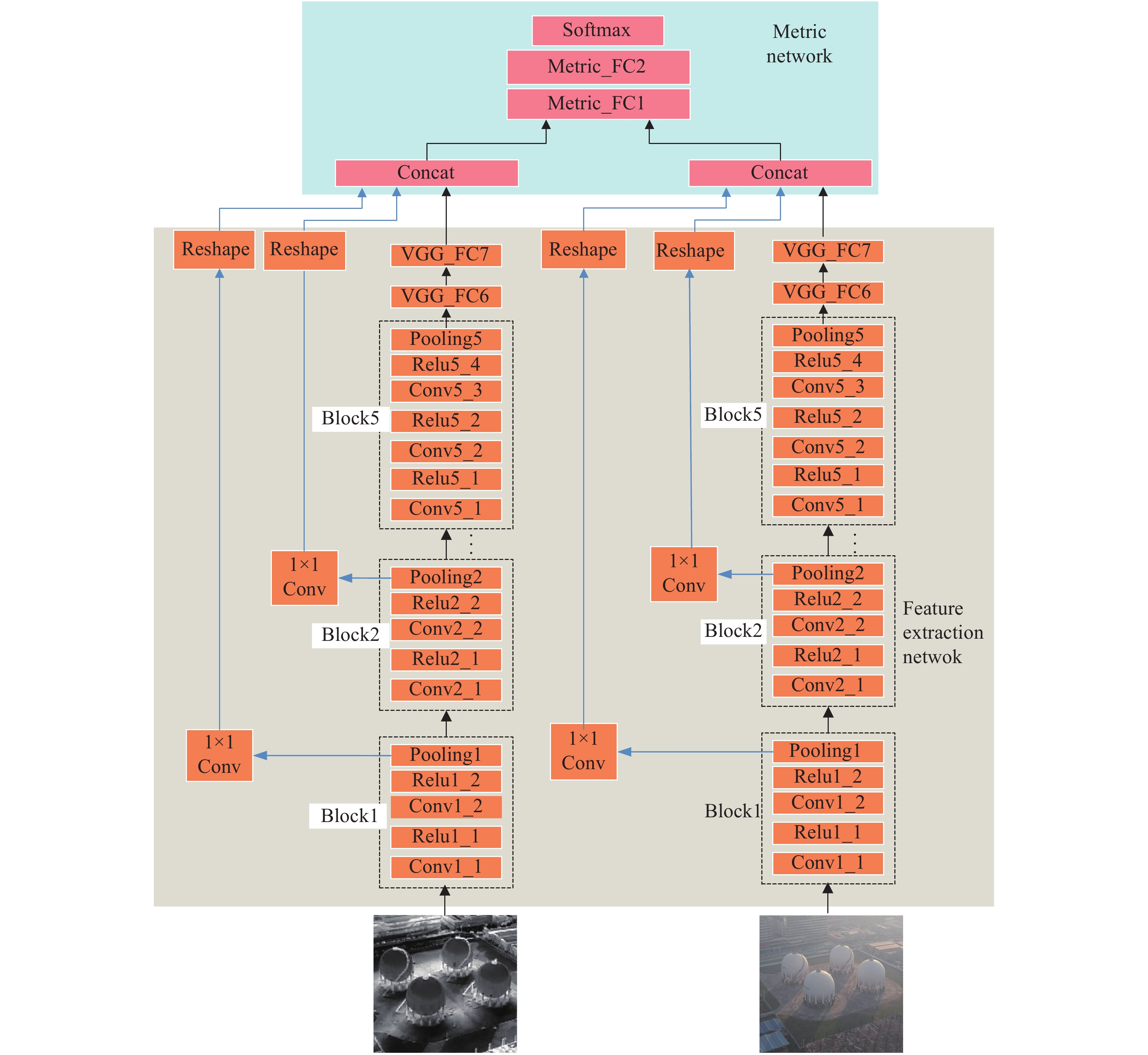
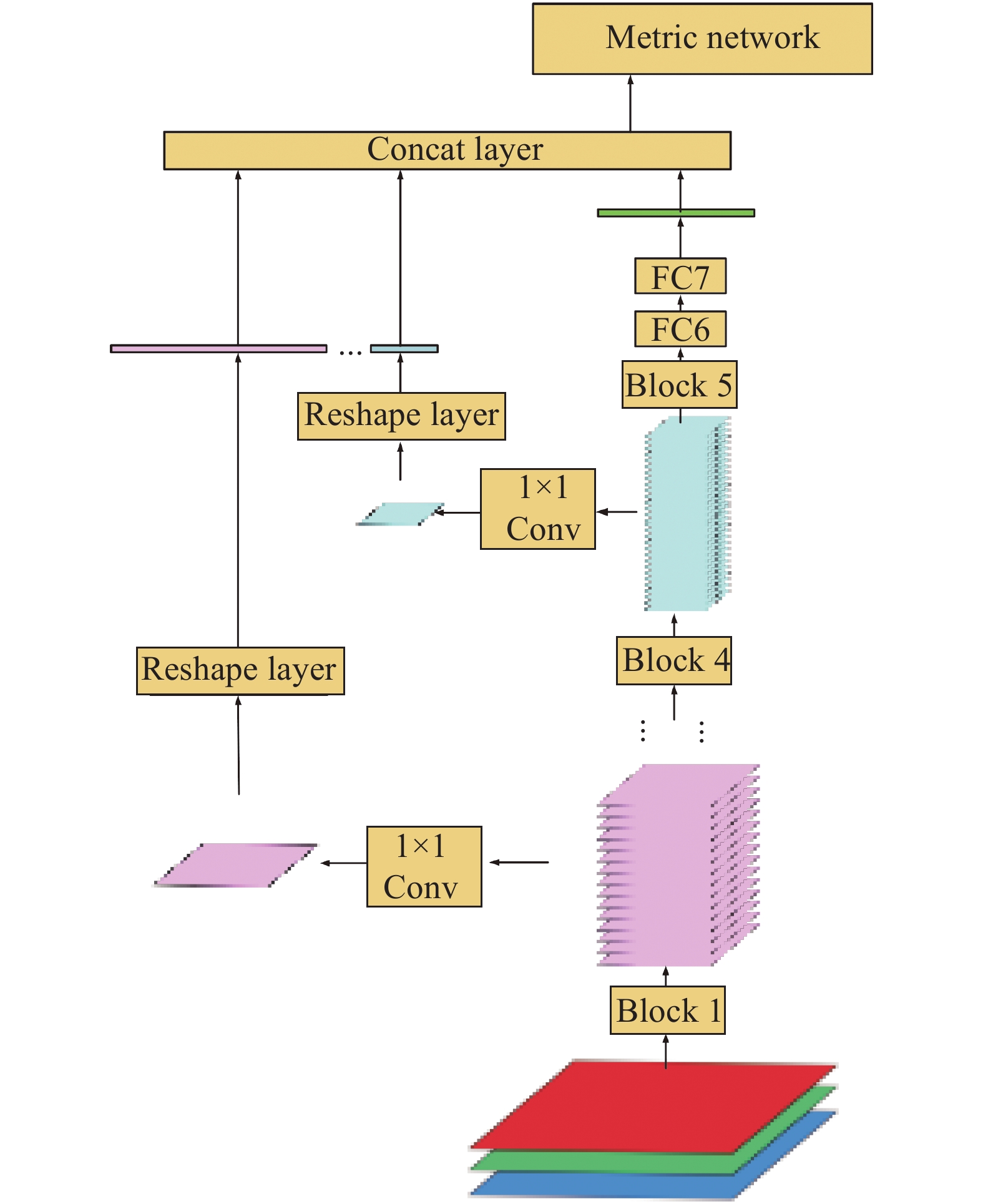
Our network mainly consists of two parts: the feature extraction network and the metric network, as shown in Fig.1. The feature extraction network is responsible for extracting features in infrared and visible images. The metric network mainly matches the feature’s similarities.
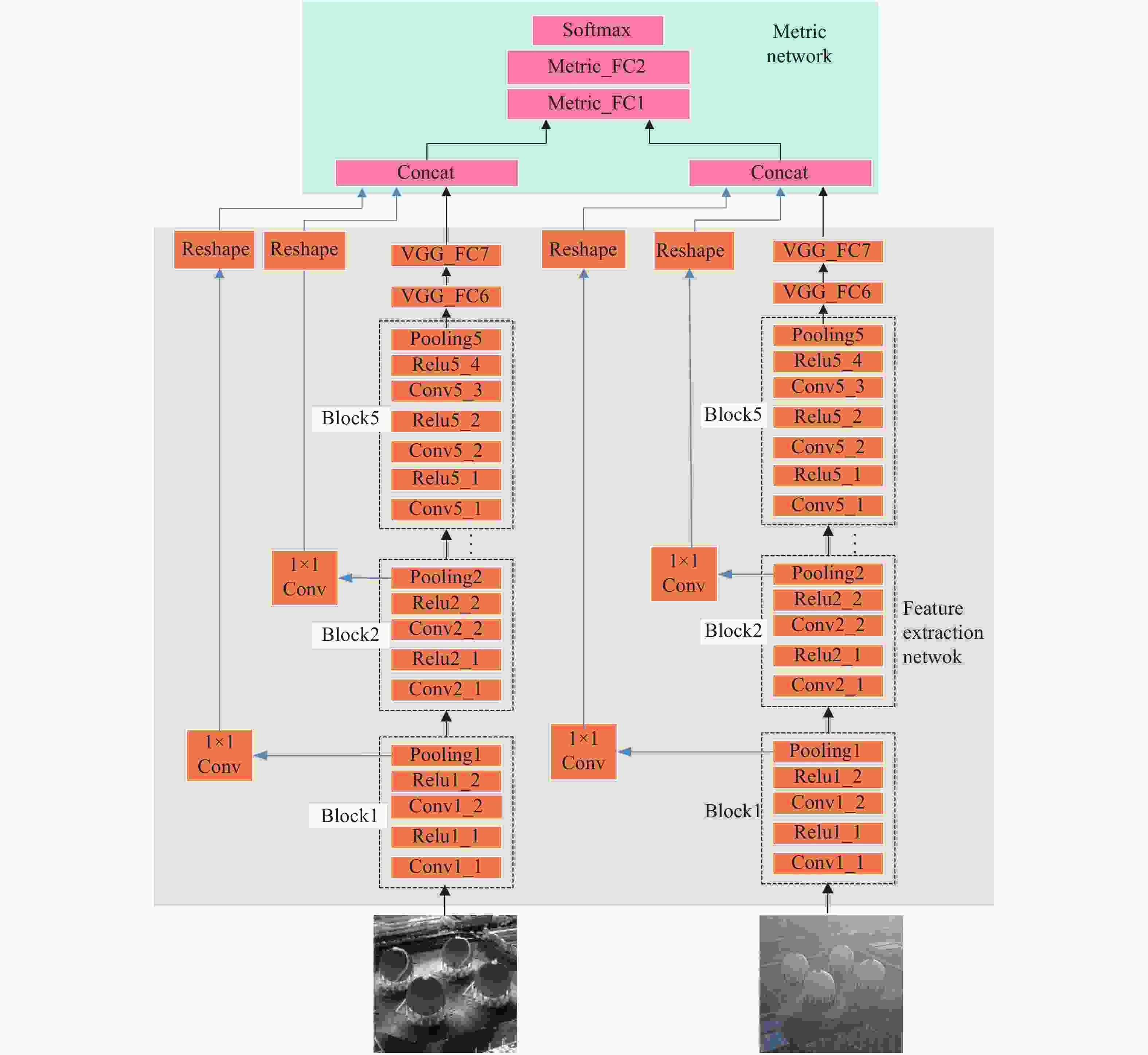
Figure 1. Infrared-visible image deep matching network. The black line with the arrow indicates the data-flow. The blue lines represent shortcut connections through the reshape layers. This figure describes the process of the infrared-visible image patches matching
The feature extraction network extracts the distinguishing features of visible and infrared images. In the feature extraction network, infrared and visible images are input into two VGG16[16] branches, which constitute a Siamese network. To be compatible with the visible image’s three channels, we copy an infrared image into three channels as another branch input. The weights are shared in the two branches. There are five blocks and two FC layers in a single VGG16 branch. A block consists of two or three convolution layers, an activation layer, and a pooling layer. In a single VGG branch, we retain the original FC6 and FC7 layers in VGG16. There are two reasons for retaining the two FC layers. Firstly, the FC7 layer can produce a feature of 1×4096 dimension, rather than 7×7×512 dimensions from the Conv5 block. It can significantly reduce the parameters and calculations in the metric network. Secondly, we find that the branch with FC layers has better performance than that without them in training.
For infrared and visible images, although their imaging principles are different, the same target is very similar in semantic features. Therefore, branches share network weights in network design. We believe that deep convolutional networks have strong feature representation capacity. It can extract common feature in infrared and visible images. Multiple network branches that traditionally use contrastive loss or triplet loss generally share weights. The shared weights can map high-level features to the same feature space for distance comparison.
The metric network is composed of two FC layers with softmax loss as the objective function. It estimates the probability of whether the visible image and the infrared image are similar or not. Ideally, if they match, the prediction is 1. If they don’t match, the prediction is 0.
-
Compared with visible images, infrared images have no color and less texture information. The edges are usually blurred. However, the objects still have rough outlines and region information in infrared images. These outlines and shapes are common features in visible and infrared images. Therefore, we believe that their spatial information is essential in infrared images for image matching. It is necessary to integrate the spatial features with the semantic features to enhance feature representation.
On the other hand, it is feasible to propose features with multiple scales in the deep neural network's hierarchical framework. The features proposed from the low-level layers are similar to those extracted with the hand-craft descriptors, such as SIFT, SURF. As the CNN layers deepen, the feature maps less focus on the imaging difference. The semantic features gradually reveal in the high-level layers. In our network, the multi-scale features are input into the metric network. So, the metric network can use more comprehensive information to make similarity decisions. Each block in our network directly connects to the input of the metric network. It can preserve more multi-scale spatial information for similarity comparison in the metric network, as shown in Fig.2.
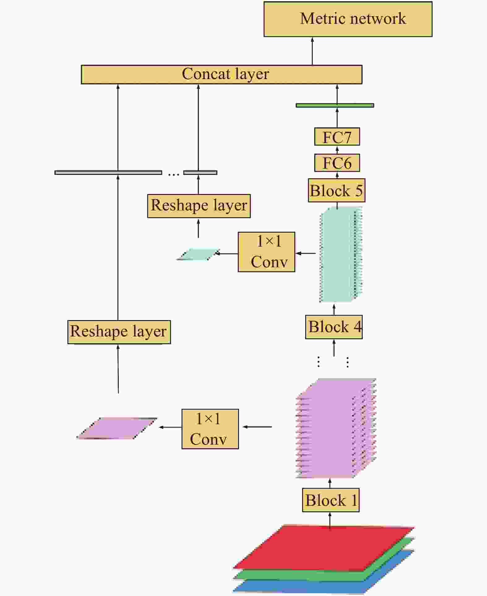
Figure 2. Multi-scale spatial feature integration in a single branch. The output feature map in each block shorts to the concatenation layer. The output of the concatenation layer is one input of the metric network
In multi-scale spatial feature extraction, two problems need to be solved. Firstly, the shortcut feature should maintain the original feature maps' size in each block to preserve spatial information. Secondly, the shortcut feature dimensions should not be too high after it reshapes into a vector. The great dimension eventually results in vast parameters and high computation in the metric network.
The 1×1 convolution is adopted in our network to solve the problems. The 1×1 convolution is widely used in GoogLeNet[17]. The multi-channel feature maps are compressed into a single-channel feature map, which preserves the spatial information and avoids the too high dimensions. To connect the features of different dimensions, they are converted to the vectors of length N×N with the reshape layer. N represents the size of the corresponding feature map. All multi-scale feature maps, including the semantic feature from the FC7, are concatenated as the input of the metric network. In the metric networks, its inputs include the infrared image branch and the visible image branch.
-
As shown in Fig.3, the network of feature extraction consists of two branches. Two branches are identical in structure and share weights. A visible image and an infrared image make up an image pair. The contrastive loss was first used for dimensionality reduction[18]. Here, the contrastive loss is used as the objective function to train the two branches.
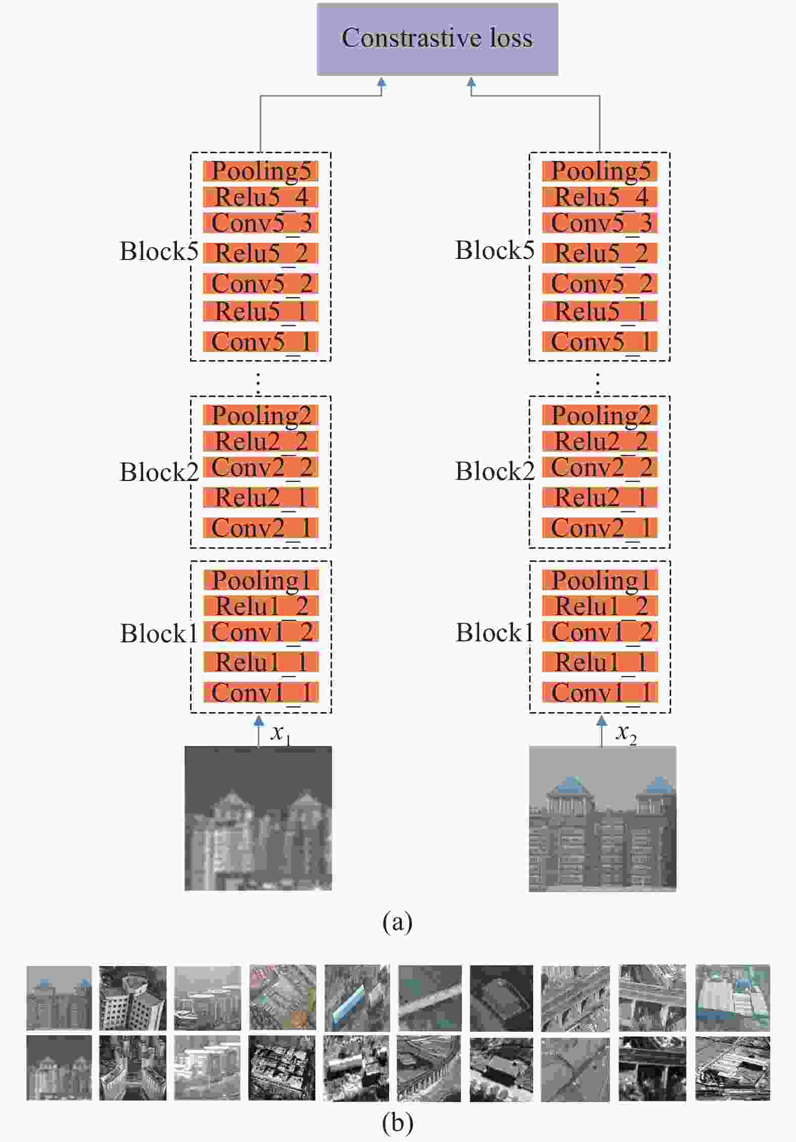
Figure 3. (a) Feature extraction network architecture with the contrastive loss; (b) Input data for feature extraction network with the contrastive loss. The visual patches are in the first row. The infrared patches are in the second row. The positive samples are in odd columns. The negative ones are in even columns
The contrastive loss is shown in Eq.(1).
where
${{d}}\mathrm(f({x}_{1}), f({x}_{2}))$ represents the Euclidean distance of two sample features;${p_1}$ is the label of input visual image;${p_2}$ is the label of input infrared image.${p_1} = {p_2}$ means a similar patches pair.${p_1} \ne {p_2}$ means an unrelated patches pair. The margin is a threshold in Eq.(1). It represents the distance that should be separated from the unrelated features, at least. In our experiment, the margin is set to 1. -
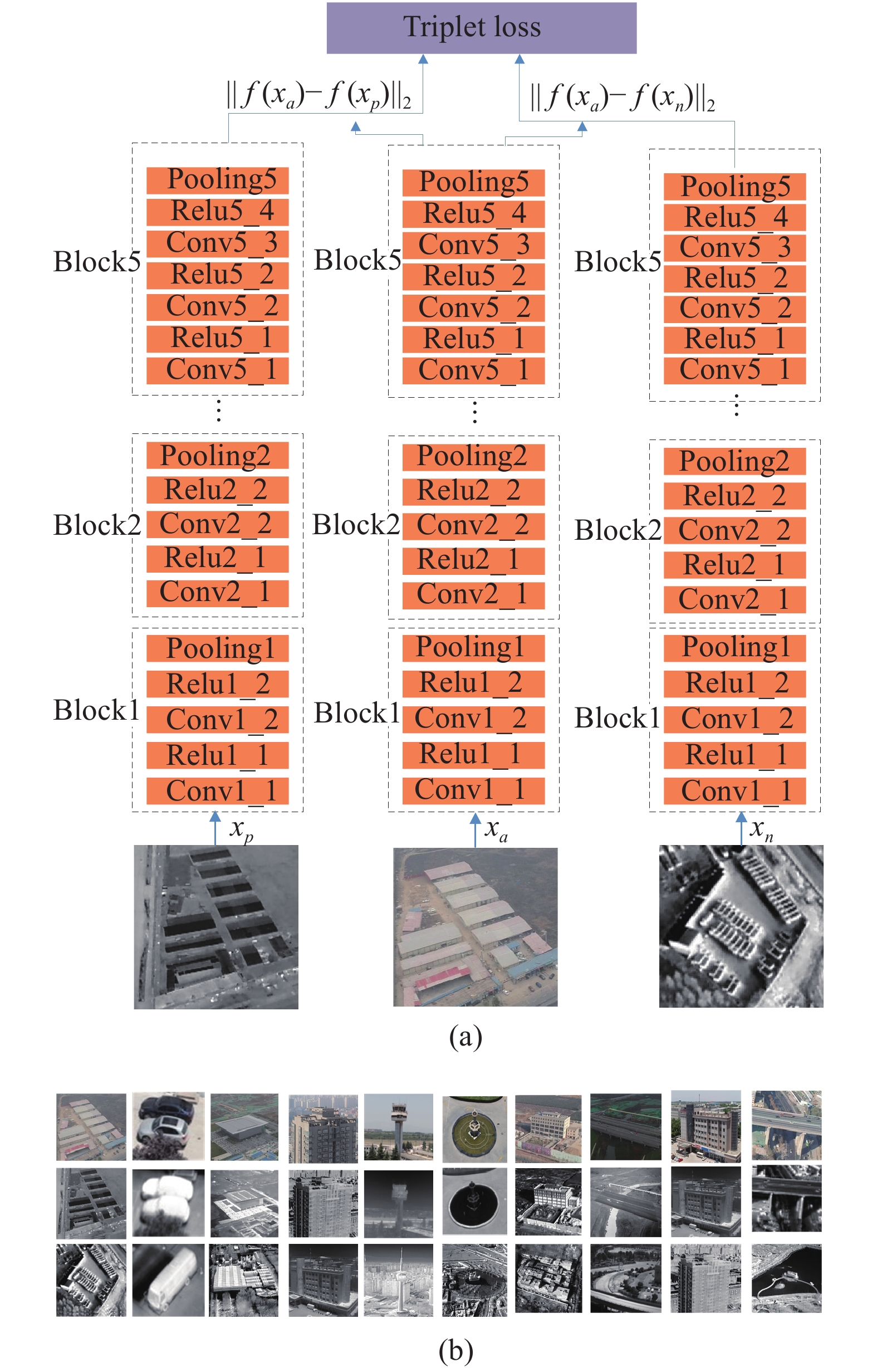
As shown in Fig.4 (a), the network consists of triple branches. Three branches are identical in structure and share weights. A visible patch (anchoring sample), an infrared patch (positive sample), and another infrared patch (negative sample) form an image pair. We input a triple pair at a time to train the feature extraction network. The triplet loss was used for face recognition[19] firstly. Here, it is used as the objective function to train the triple branches.
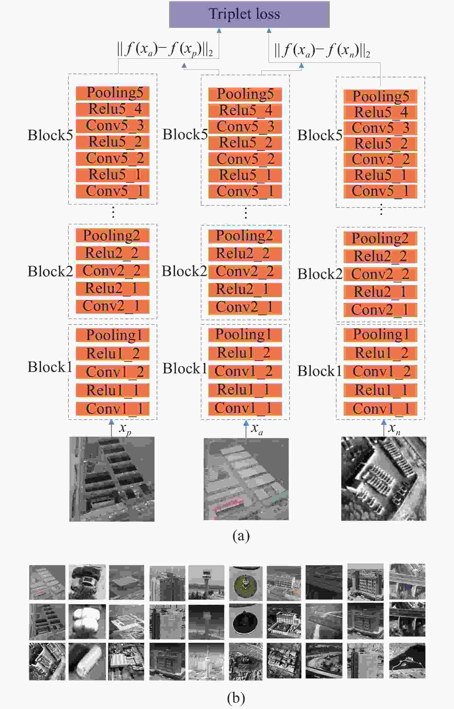
Figure 4. (a) Feature extraction network architecture with the triplet loss; (b) Input data for feature extraction network with the triplet loss. The anchor patches are in the first row. The positive patches are in the second row. The negative patches are in the third row. Each column is triple patches input
The triplet loss shows in Eq.(2).
The input data include anchoring sample (
${x_a}$ ), positive sample (${x_p}$ ) and negative sample (${x_n}$ ).${d}(f({x_a}),f({x_p}))$ represents the Euclidean distance of the anchoring sample and the positive sample.${d} (f({x_a}),f({x_n}))$ represents the Euclidean distance of the anchoring sample and the negative sample. By optimizing the function, the distance between the anchoring example and the positive example is less than the distance between the anchoring example and the negative example. The anchoring example is randomly selected from the sample set. The positive example and the anchoring example go to the same class, while the negative example and the anchoring example belong to different classes.Eq.(3) illustrates that there is a margin between
${d(}f({x_a}),f({x_p}))$ and${d(}f({x_a}),f({x_n}))$ to distinguish positive and negative samples. Unlike contrastive loss, the triplet loss function compares the distance between positive and negative samples in a forward and backpropagation process. Compared to visible image matching, the same object’s imaging difference is also relatively large in multi-source image patches matching. So, it is found that a larger margin can achieve better performance in our experiment. The margin is set 3 to achieve the best performance. -
There are no available infrared-visible image patches matching datasets on the Internet, so we have to collect image pairs ourselves. In data acquisition, the visible camera is the default equipment in the DJI UAV. The infrared camera is manufactured by FLIR company. The wavelength of the infrared camera ranges from 7.5 to 13.5 µm. In terms of image resolution, the UAV acquires infrared and visible images at different altitudes. In the original image, the proportion of the same target to the image size is 0.8×, 0.5×, and 0.25×, respectively. In the following data preprocess, we crop the target area from the original images. The input images of the neural network resize to 224×224. Therefore, we use different resolution images during training and testing.
Our data set contains 2 000 images, falling into 25 classes. For scene selection, the target taken by UAVs should be different in shape and outline. The classes cover bridges, buildings, roads, parking lots, factories, houses, towers, gas storage tanks, etc., as shown in Fig.5. In the data set, the ratio of visible and infrared images is 1∶1. 80% of the images are used as training data. The rest images are used as test data. A sample includes an infrared patch and a visible patch. If the image pairs are similar, they are positive samples. Their ground truth is 1. If they are not similar, they are negative samples, and the ground truth is 0. In the training and test data set, the ratio of positive and negative samples is 1∶1.

Figure 5. Infrared-visible image samples. Ten image pairs randomly was selected. The ground truth of the first five images is 0. The ground truth of the last five columns is 1
-
InViNet using two-stage training is better than the traditional classification network. In two-stage training, the feature network can improve the features representation. It can significantly increase the accuracy of the metric network in the latter stage. By comparing the existence of shortcut connections in InViNet, the low-level spatial feature is acknowledged as a useful complement for high-level semantic information. We use the following settings to train our network in two stages.
The feature extraction network is trained in the first stages. The branches in the feature extraction network are initialized with VGG16 trained weights by the ImageNet data set. Xavier[20] method initializes the new or modified layers. The low-level filters in VGG16 are acknowledged that they are beneficial for the shallow features, while higher-level features are more closely related to specific tasks. So, the learning rate multipliers in each layer are also set differently. The learning rate in each layer is the basic learning rate multiplied by its learning rate multiplier. The basic learning rate is 10−3. The learning rate multiplier is 0.01 in Block1, Block2, and Block3. The learning rate multiplier is 0.05 in Block4 and Block5. The learning rate multiplier of FC6 and FC7 in VGG remains 1. Since all branches share weights, only one copy of the weights is in the feature extraction network. The optimizer uses the momentum SGD method. The momentum parameter is 0.9. Minibatch size in training is 16. The number of epochs is 2 000. The weight decay is 10−4.
The metric network and shortcut connections are trained in the second stage. In metric network training, the weights trained well in the feature network are used as the initial value. The branches' weights slightly change during this training. Their learning rate multipliers are less than 10−2. The basic learning rate is 10−3. The weights are initialized with the Xavier method in new layers. Their learning rate multipliers are 1 in the metric network and shortcut layers. The number of epochs is adjusted to 2 500. The rest of the training parameters are the same as the first training.
All experiments run on a computer equipped with Nvidia TITAN XP GPU. Our experiment is implemented with Caffe.
-
To validate our approach, we have implemented the following experiments on different network architecture.
(1) Traditional method[9]. We enhance the object edges and use SURF to extract the infrared-visible image features. The similarity of images is measured by matching the feature points of the infrared and visible images.
(2) Baseline Network. MatchNet[13] is used as a baseline network. The Softmax loss function directly optimizes the whole network. There are no two phases in training. Two VGG16 branches train from scratch. The network has been over-fitting soon.
(3) MatchNet[13](F). MatchNet architecture improved with fine-tuning. Unlike the baseline network, its VGG16 branches are initialized by the weights trained with the ImageNet dataset.
(4) Pseudo-SiamNet[14] (F). The pseudo-Siamese Deep Compare Network architecture improved with fine-tuning. In the two VGG16 branches, the Conv1, Conv2 and Conv3 layers use their respective weights, whereas the Conv4 and Conv5 layers share the weights. The model weights also are initialized by the VGG16 trained to avoid over-fitting.
(5) InViNet (F+C). InViNet with fine-tuning and contrastive loss. We trained this network in two phases, which are described in Sec 2.2.
(6) InViNet (F+C+S). InViNet with fine-tuning, contrastive loss, and shortcut connection. The network adds shortcut connections.
(7) InViNet (F+T+S). InViNet with fine-tuning, triplet loss, and shortcut connection. This network is mainly to compare triplet loss and constrained loss.
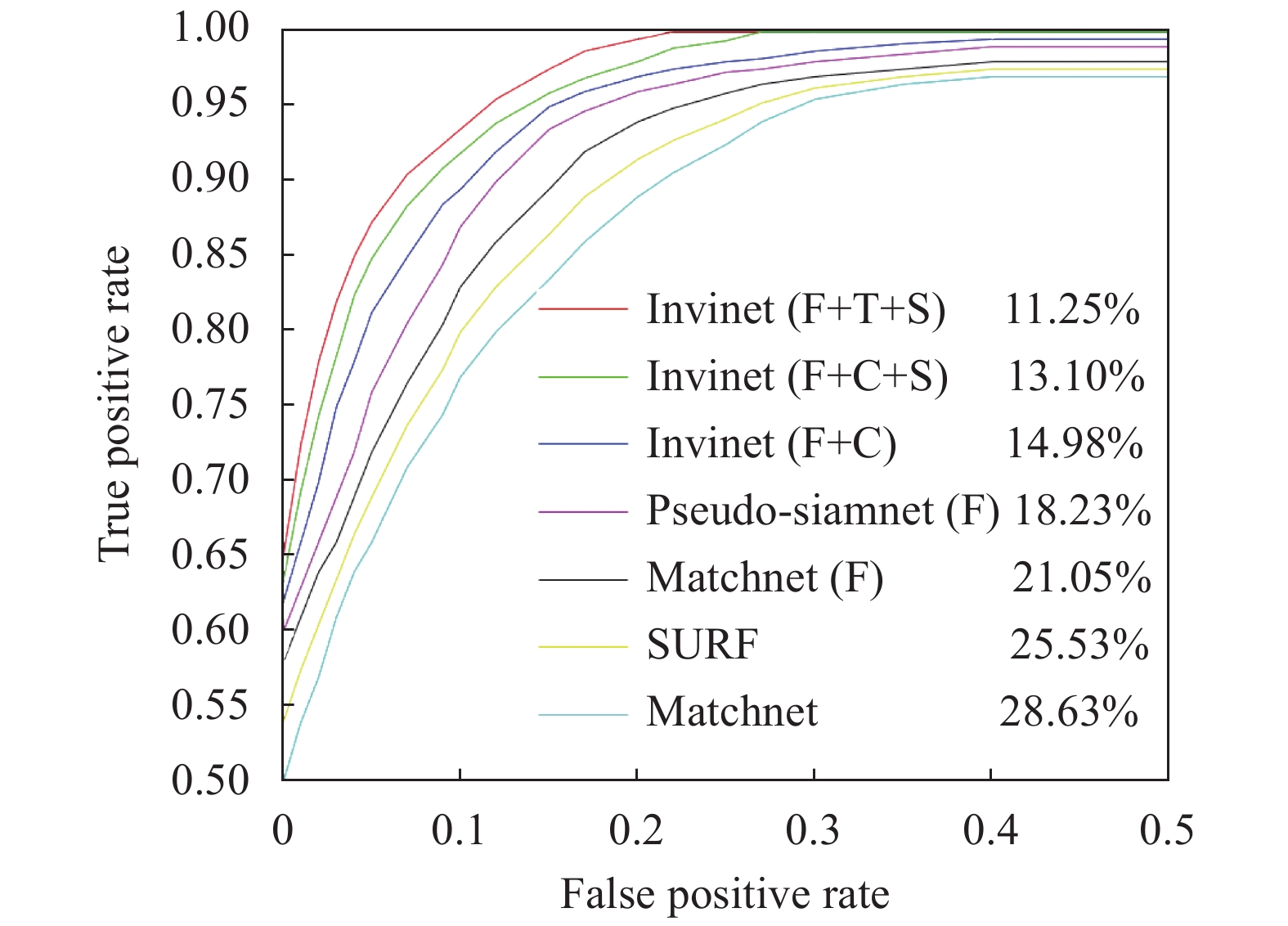
The ROC curve usually measures a binary classification performance to avoid the imbalance between positive and negative samples. The commonly used evaluation metric is the false positive rate at 95% recall (Error@95%), the lower the better. Based on the experimental results, ROC curves are drawn for different methods. See Fig.6 for details.
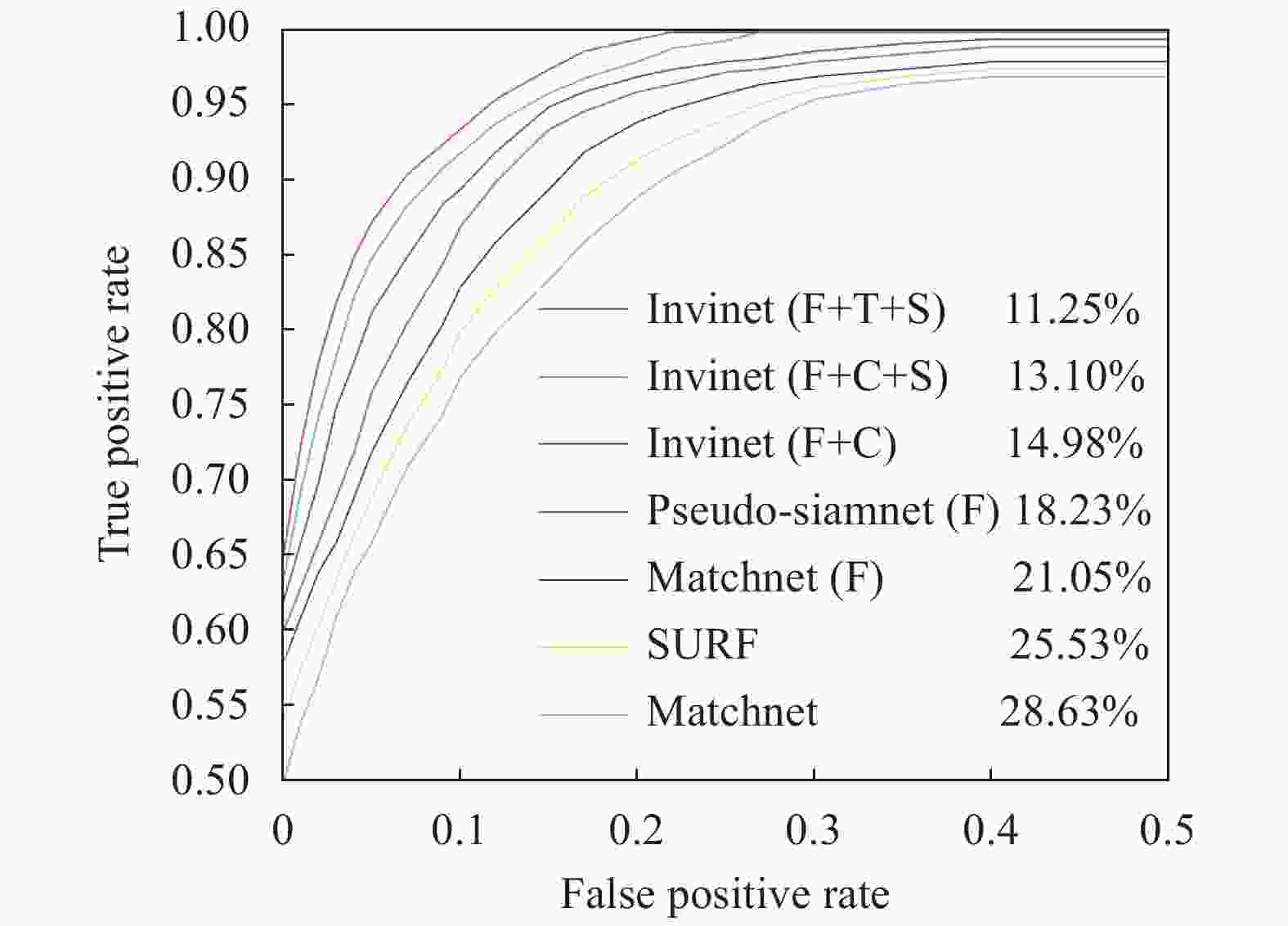
Figure 6. ROC curves for various methods. The numbers in the legends are FPR95 values. In the legend, the symbol “F” means the network uses fine-tuning with VGG16. The symbol “C” means that the contrastive loss is used in the extraction feature network. The symbol “T” means that the triplet loss is used in the extraction feature network. The symbol “S” means that shortcut connection is used
From our experiments, the following conclusions can be summarized.
(1) In infrared-visible image patches matching, it is hard to extract common features in infrared and visible images with traditional methods due to the different imaging principles. The result is not satisfying.
(2) The few samples easily lead to over-fitting when the network is trained from scratch. With the fine-tuning, all deep learning networks show better performance than traditional algorithms. The fine-tuning can avoid over-fitting effectively.
(3) The pseudo-Siamese network performs better than the Siamese network. The explanation may be that the low-level convolution layers don’t share weights in pseudo-Siamese networks. According to the different imaging principles of infrared and visible images, they can extract their unique shallow features from two separate branches.
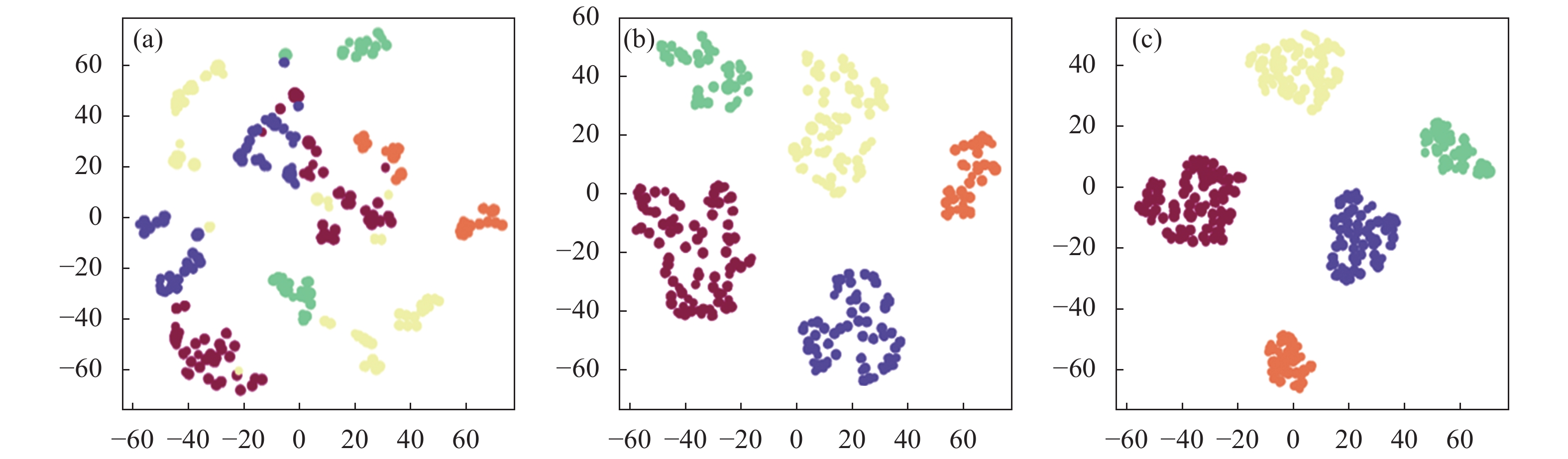
To be concrete, we visualize the deep learned features of expression using t-SNE[21], a common tool used to visualize high-dimensional data. Our approach can effectively reduce the intra-class distance and enlarge the inter-class distance in Fig.7 which is beneficial for patches matching.
We show some top-ranking correct and incorrect results in InViNet in Fig.8. We find that incorrect results also may be easily mistaken by a human.

Figure 8. Top-ranking false and true results in overpass and factory image patches. (a) True positive samples; (b) True negative samples; (c) False positive samples; (d) False negative samples
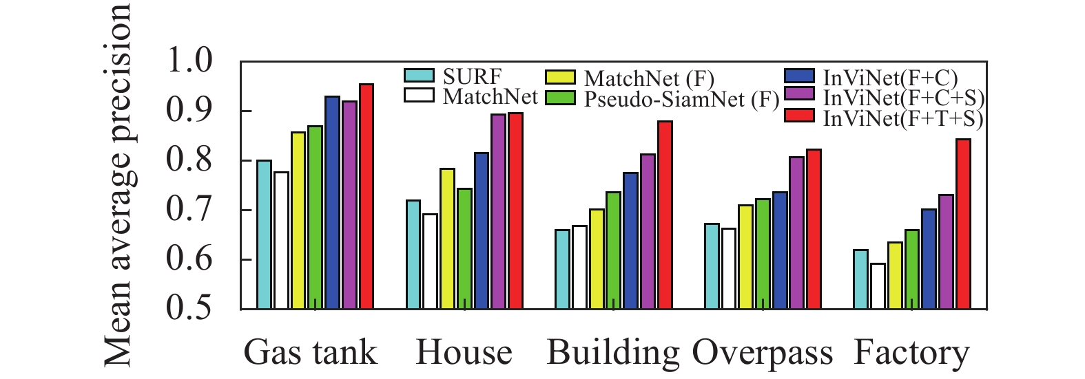
To further analyze our method results, we list the mean average precision (MAP) in the test set, which has five classes. The classes have never been used in the training process. As shown in Fig.9, our InViNet outperforms other approaches.

Figure 7. Visualization of the five class features in the test data set by the feature extraction network. (a) Features from the original network; (b) Features from the network with the contrastive loss; (c) Features from the network with the triplet loss
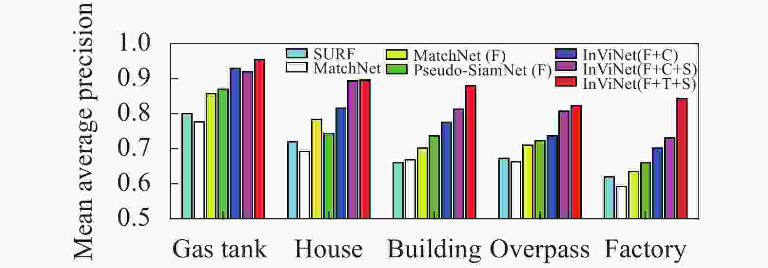
Figure 9. Performance matching in the test data set. In the legend, the symbols “F”, “C”, “T” and “S” have the same meaning in Fig. 6
-
Given the difficulty of infrared-visible image patches matching, this paper proposes an improved network based on deep learning. Compared to the previous method, our method can increase the accuracy from 78.95% to 88.75%. At present, it is difficult to obtain samples of visible and infrared images. There are many multi-sensor data sets available on the Internet. However, they are not fully utilized because there is no corresponding similar visible image. We believe that we can make full use of many multi-sensor images through unsupervised learning to further improve our matching performance in the future.
Infrared-visible image patches matching via convolutional neural networks
doi: 10.3788/IRLA20200364
- Received Date: 2020-09-20
- Rev Recd Date: 2020-11-04
- Publish Date: 2021-05-21
-
Key words:
- infrared-visible image patches matching /
- convolutional neural networks /
- contrastive loss /
- triplet loss /
- multi-scale spatial feature integration
Abstract: Infrared-visible image patches matching is widely used in many applications, such as vision-based navigation and target recognition. As infrared and visible sensors have different imaging principles, it is a challenge for the infrared-visible image patches matching. The deep learning has achieved state-of-the-art performance in patch-based image matching. However, it mainly focuses on visible image patches matching, which is rarely involved in the infrared-visible image patches. An infrared-visible image patch matching network (InViNet) based on convolutional neural networks (CNNs) was proposed. It consisted of two parts: feature extraction and feature matching. It focused more on images content themselves contrast, rather than imaging differences in infrared-visible images. In feature extraction, the contrastive loss and the triplet loss function could maximize the inter-class feature distance and reduce the intra-class distance. In this way, infrared-visible image features for matching were more distinguishable. Besides, the multi-scale spatial feature could provide region and shape information of infrared-visible images. The integration of low-level features and high-level features in InViNet could enhance the feature representation and facilitate subsequent image patches matching. With the improvements above, the accuracy of InViNet increased by 9.8%, compared with the state-of-the-art image matching networks.


 DownLoad: