High-resolution satellite ocean background imaging simulation method

近年来，利用高分辨率卫星影像对海面目标进行探测、发现和识别是遥感技术的一个重要应用方向^[1-2]。然而，公开可获取的高分辨率海洋舰船目标遥感图像较少，且难以覆盖不同海况、不同天候、不同目标和不同观测几何的各种情况。海洋目标场景仿真可为舰船目标检测识别算法的研究和验证，提供不同条件下的完备数据样本。

海洋场景仿真中，海洋背景仿真是关键环节，是海洋目标-背景耦合作用模拟的重要基础，决定了仿真图像中目标与背景差异特征的正确性和真实性。例如在高分辨率遥感影像中，海面起伏造成零星分布的耀斑，以及海浪泡沫形成的白帽等也可分辨，尺度与舰船目标近似，遥感器对其响应亮度值近似或高于舰船目标^[3-4]。因此，对于高分辨率海面遥感仿真，传统将海面视为单一均匀辐射面，仿真图像不能正确表征海面高分辨辐射特征，更无法准确刻画目标与背景的特异性，大大减低了仿真结果的应用效果。

目前，海面背景仿真的相关研究主要集中在海面三维模型和辐射特性两个方面。针对海面的三维模型，Fournier将Gerstner海浪数值模型应用到海浪的可视化中，提出海面水质点绕着固定位置做椭圆运动，引入海底深度参数，实现较真实的海浪场景^[5]；郑茂琦基于随机震动相关理论，提出了改进海朗普的海浪模型，解决了波峰及波谷变化突兀的问题^[6]；Lima基于几何形状构建了卷浪模型，并将其嵌入海洋场景中，实现了浅海浪的仿真^[7]。但上述的研究内容还停留在模拟海浪的几何结构及视觉效果上，并没有考虑海浪的光学辐射特性。在海面辐射特性研究方面，唐军^[8]等基于蒙特卡洛模拟方法，构建了标量的水体辐射传输模型，并用该模型分析了离水辐射的方向性分布特征。张鉴^[9]等基于矩阵算法，建立了标量的航洋-大气耦合辐射传输模型，并模拟了水色遥感参数的变化特性。但他们在考虑海面对太阳和天空背景辐射的散射和海面自身辐射时，多将海面视为均匀辐射面，忽视了海面三维结构动态变化的特性，以及该变化所带来的辐射调制作用^[10]。

在目标可辨识尺度下，海面三维特性突显，起伏表面调制海水辐射特性，呈现其辐射场特有的空间分布特性及图像特征。

文中研究了海况与海面几何特征的关联规律，建立了三维海浪模型，重点研究了三维海面对海水辐射特性的调制作用，建立了亚米级尺度的海面三维辐射特性模型，并根据不同光照和观测条件，利用光线追踪计算海面零视距辐射分布场。同时，模拟了三维海面反射的大气辐射传输和邻近效应作用，以及传感器系统调制，得到不同海况下高分辨率卫星海面成像结果，可以为海面目标检测效能评估提供有力的数据支撑。

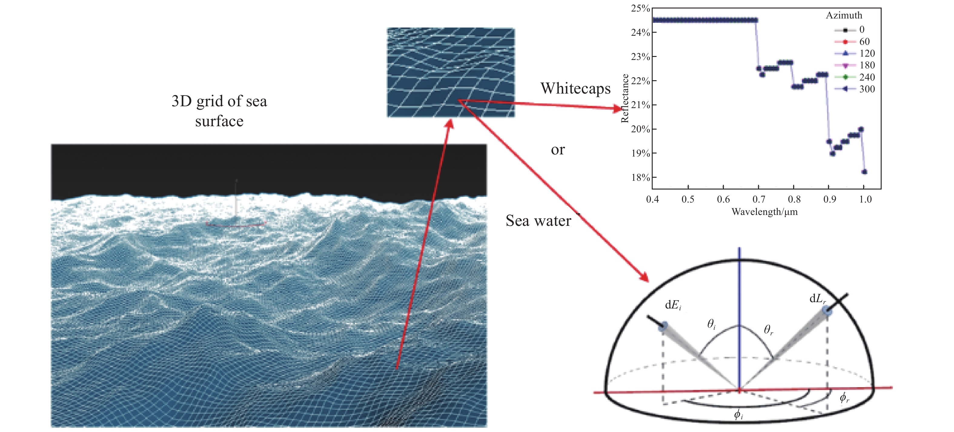
高分辨率卫星观测下的海洋背景与低分辨率卫星不同，随着海表分辨率的提高，海面细节得以显现。因此，需要考虑因海面风力变化导致的海面起伏及白帽分布变化，结合海水的三维几何、组分分布及各组分辐射信息来构建高精度的三维海面辐射模型。建模构型如图1所示，海面三维辐射模型由海面的三维几何模型与海水的各组分方向反射特性两部分组成，海水的各组分方向反射信息依托于构成海面三维几何的网格面片而存在，以面片的法向为基准反射方向。其中各组分的方向反射信息可以由叶绿素浓度、海水含盐量、太阳角度、观测角度以及风速风向等参数进行计算得到，海面的三维几何构造及各组分分布则可以根据海面的风速风向及海浪级别进行三维几何建模。

Figure 1.  3D radiation model structure diagram of the sea surface

海浪的形成可由不同的物理理论来解释，但总体可以看作是大气到海洋的能量传递，海浪从生成到消退的过程可以看作是能量的摄取与消耗。风本身的运动又是复杂多变的，其产生的海浪无论是在时间上还是空间上都具有不规则性和不重复性^[11]。对于充分成长的海浪，在一段时间内认为它是平稳随机过程是足够精确的。从海洋学理论出发，用频谱函数描述海浪的表面，经傅里叶变化实现海浪的动态模拟，可以很好的体现海浪的随机性，同时也是海浪研究中应用最广泛的方法。采用基于FFT(Fast Fourier Transform)的频谱分析方法，根据海面的实测风速，通过计算海浪的频谱函数得到多个频率、振幅对应的正余弦波，并利用FFT算法计算空间域下的海浪顶点高度^[12]。X=(x,y)表示海面网格上的一点，其在t时刻的高度记为h(X,t)，则其表达式为：

式中：波数向量K=(k_x,k_y)=(kcosθ, ksinθ)，k=|K|=$\sqrt {k_x^2 + k_y^2} $，其中θ为向量K与x轴正半轴的夹角；$\tilde h(K,t)$表示振幅的傅里叶分量。

h(X,t)通过IFFT(Inverse Fast Fourier Transform)将波幅从波数域K转换到位置域X，可以通过位置和时间计算出波幅：

式中：*表示复数取共轭；${\varepsilon _r}$和${\varepsilon _i}$为均值为0方差为1的高斯随机数；Ph(K)为Phillips谱，即：

式中：A为常数；$L = {U^2}/g$；u=(Ucosα,Usinα)，U为风速大小，α为风向。

根据海况表的描述见表1，利用上述的海浪模型模拟不同级别海浪的三维构造。将不同海浪等级对应的海面风速及风向参数代入公式(3)中，得到对应的Phillips谱Ph(K)，再将Ph(K)代入公式(1)和(2)中，得到海面上任一位置X(x,y)在t时刻的高度h(X,t)。利用海浪网格模型生成面片数为1 024×1 024，单元尺寸大小为0.5 m的海面三维网格模型。

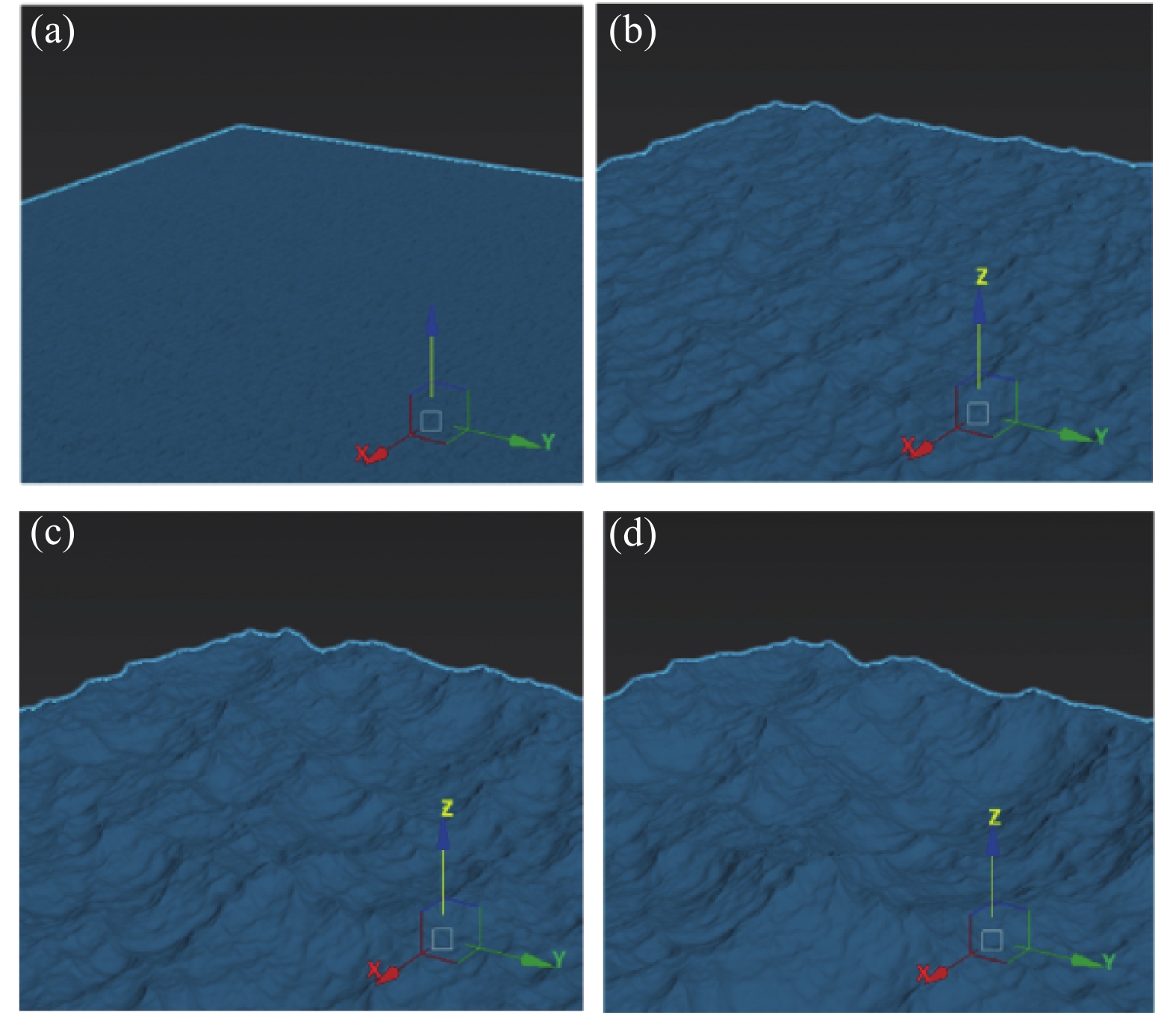
在光学遥感影像中，具有实际应用价值的影像多是在无云晴好的天气下拍摄。这种天气对应的海况等级相对较低，所以文中主要对海面1~4级海浪进行模拟。图2为根据上述方法模拟的海面三维结构图。

Figure 2.  3D structure of the sea surface under different sea conditions. (a) Level 1 sea state; (b) Level 2 sea state; (c) Level 3 sea state; (d) Level 4 sea state

为了确定上述海面三维网格模型中每个面片的方向反射信息，需要构建逐面片的海面三维辐射模型。根据Koepke在参考文献[13]中的描述，低分辨率情况下，在太阳光谱范围内，对于给定的一组几何条件太阳天顶角θ_s，观测天顶角θ_v和相对方位角φ(=φ_s−φ_v)，海面的反射率${\;\rho _{os}}({\theta _s},{\theta _v},\varphi ,\lambda )$可以总结为白帽反射${\rho _{ef}}(\lambda )$，海表的镜面反射$\;{\;\rho _{gl}}({\theta _s},{\theta _v},\varphi ,\lambda )$及海水中的散射反射${\;\rho _{{\rm{sw}}}}({\theta _s},{\theta _v},\varphi ,\lambda )$三部分，分别乘以各自的占比权重组成。

在高分辨率遥感图像中，因具备了将水面白帽及水体区分开的分辨能力，再以这种加性的方式将白帽与水体部分反射进行混合的方法将不再适用。需要分别获取海面各组分的反射信息，构成海面辐射模型。其中，一方面要考虑白帽分布的不同引起的反射分布不同，另一方面需要考虑由于海面三维起伏引起的辐射调制作用，导致的辐射差异。所以高空间分辨率下海水的反射率因如公式(4)所示：

式中：$\vec r$为海面(x,y)处面片的法向向量；Q(x,.y)是一个返回值为布尔类型的变量，即等于0或1，用来判断海面上(x,y)坐标面片是否为白帽覆盖。当该面片为白帽覆盖时，Q(x, y)=1；当该点非白帽覆盖时，Q(x,y)=0。而取值0或1则使用白帽覆该的相对面积W来生成一个伪随机数概率确定。W可以通过风速计算得出^[14]，$W = {2.951\;0^{ - 6}}\;{{w}}{{{s}}^{3.52}}$，ws为风速，单位m/s。

海水和水面白帽的反射率由于难以利用光谱测量手段实地获取，因此，反射率光谱数据使用6S (Second Simulation of the Satellite Signal in the Solar Spectrum)中OCEABRDF模型计算获得，见表2。该模型通过输入风速风向、海水含盐量、叶绿素浓度及太阳和观测角度，可以得到白帽、耀斑及水体的有效反射率光谱。利用OCEABRDF模型，分别计算了不同观测角及方位角度下，组成海面辐射的白帽、水体及耀斑的反射率值。具体计算方法参考文献[15]。其中计算所需要的风速及风向参数可以从Weather Underground (www.wunderground.com)网站获取，叶绿素浓度值可从同时过境的MODIS (Moderate Resolution Imaging Spectroradiometer)的二级数据中获取，海水的含盐量可以从中国Argo (Array for real-time geostrophic oceanography)实时海洋观测网获取(www.argo.org.cn)。

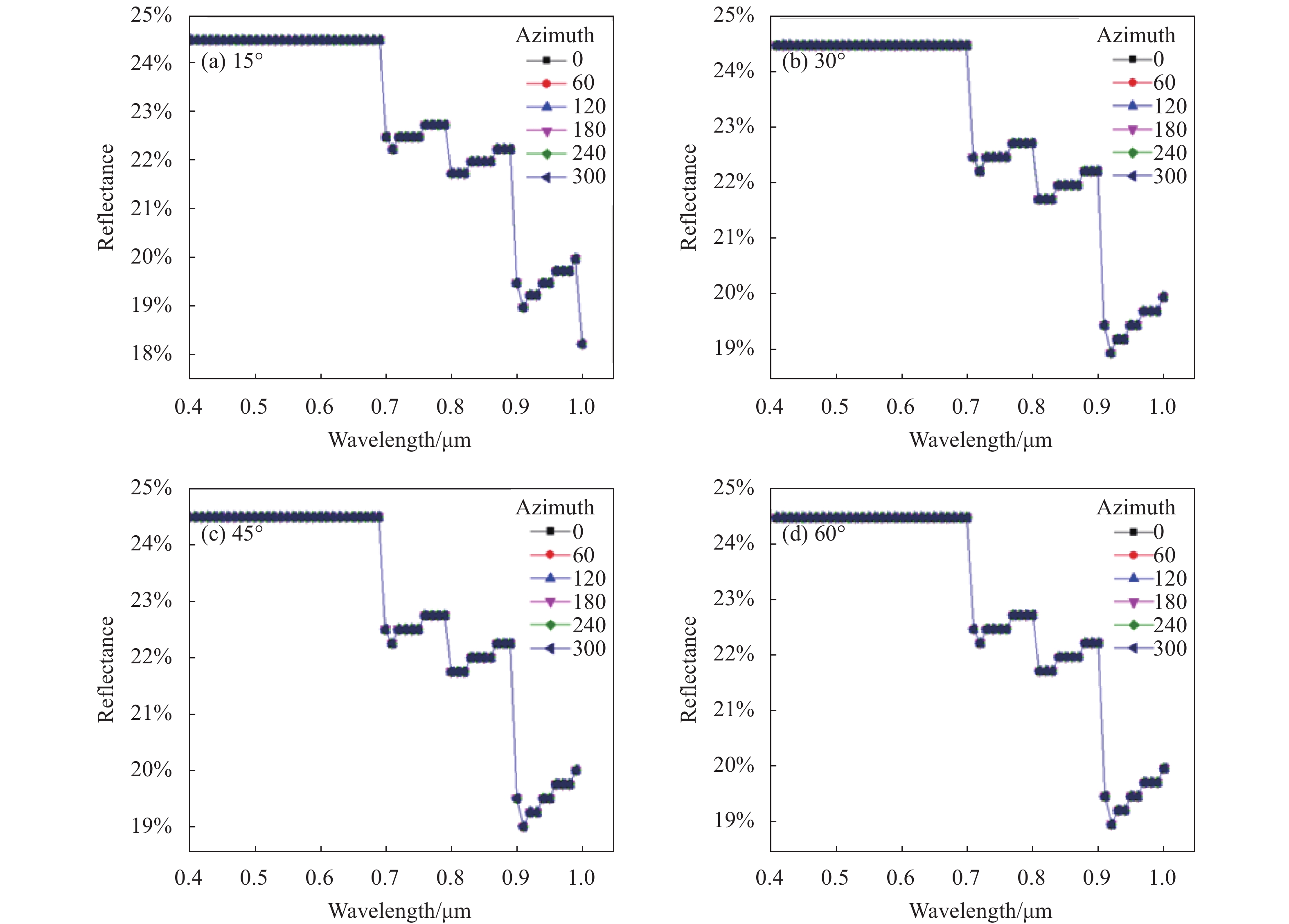
通过计算获取了无白帽覆该部分海面水体的方向反射信息，如图3所示。即公式(4)中Q(x,y)=0时，海面(x,y)处在太阳天顶角为56.6°，太阳方位角为160.4°时的水体方向反射信息${\;\rho _{os}}(x,y,{\theta _s}, {\theta _v}, \varphi ,\lambda , \mathop r\limits^{\rightharpoonup} )$。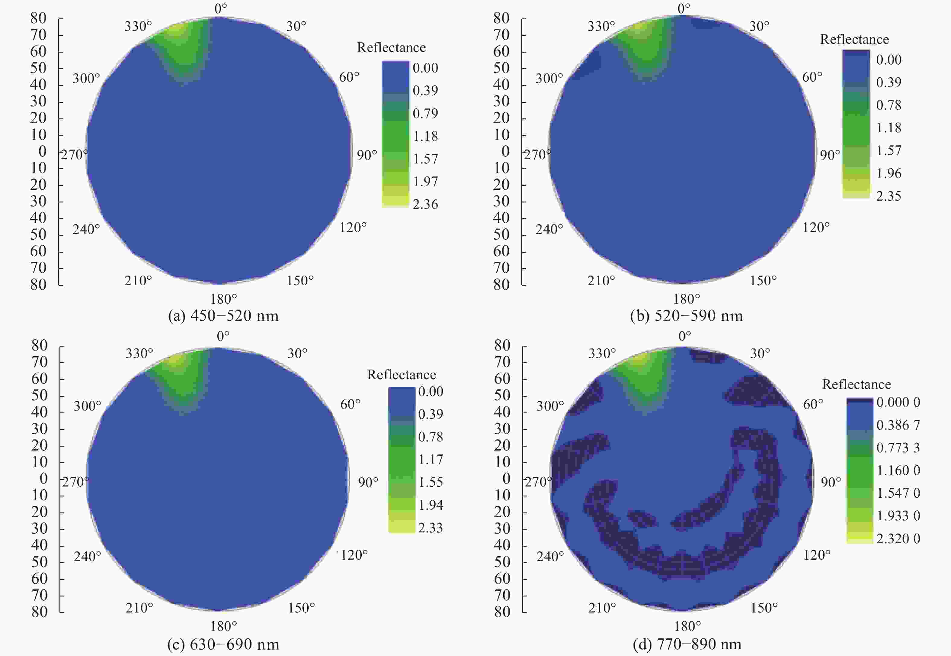

Figure 3.  BRDF of seawater at different wavebands calculated by 6S

白帽的产生是因为风破浪所产生的水体空化现象。在低分辨率遥感探测时，根据Koepke^[13]的描述，白帽的光学影响ρ_wc(λ)是由白帽的相对面积W与其对应的反射率的乘积给出的。

在高分辨率下，这里乘以白帽的面积占比给出综合反射率的情况已经不再适用，利用6S计算出不同天顶角及方位角观测时白帽的反射率，然后根据公式(5)计算出白帽的本征反射率ρ_ef(λ)。将风速8 m/s代入公式(5)，得：

计算结果如图4所示，即Q(x, y)=1时，海面(x,y)处的水体反射率信息${\;\rho _{os}}(x,y,{\theta _s}, {\theta _v},\varphi ,\lambda ,\mathop r\limits^{\rightharpoonup} ) = {\rho _{ef}}(\lambda )$。图中表示在不同观测天顶角及观测方位角下的白帽反射率数据。可以看出，不同观测方位角的反射率光谱基本重叠，不同天顶角的观测结果也基本一致。由此得出结论：在可见光范围内，白帽在不同天顶角与不同方位角上的反射率基本相同，可近似看成朗伯体。这与公式(5)中，白帽的反射率${\;\rho _{ef}}(\lambda )$只与波长λ相关的特性描述相符。

Figure 4.  Reflectivity of the whitecaps at different zenith and azimuths angles

根据海面三维几何面片网格，以及各面片材质类型（海水或白帽）和相应的方向反射特性，构建了最终的海面三维辐射模型，如图5所示。

Figure 5.  Patch type judgment

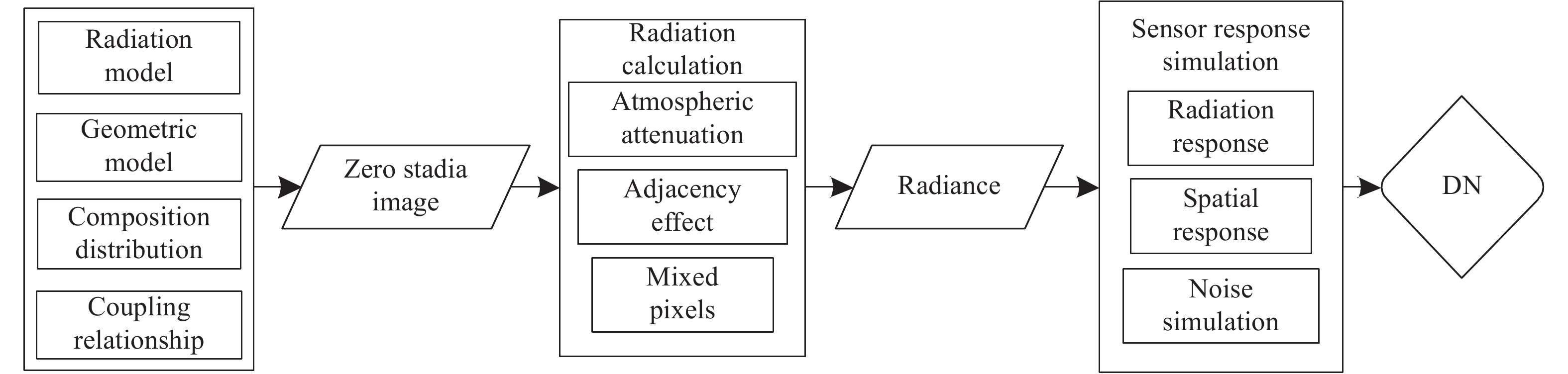
高分辨率海面成像仿真，首先是根据第1节所述的海面三维辐射模型，根据光照和观测条件计算海面出射辐射分布（或零视距辐射分布），再利用蒙特卡洛方法模拟大气邻近效应，再扣除大气的衰减，模拟混合像元，得到卫星入瞳处的辐亮度分布，最后模拟传感器的光谱及空间响应，得到仿真结果，即遥感器最终输出图像^[16-17]。整体流程如图6所示。

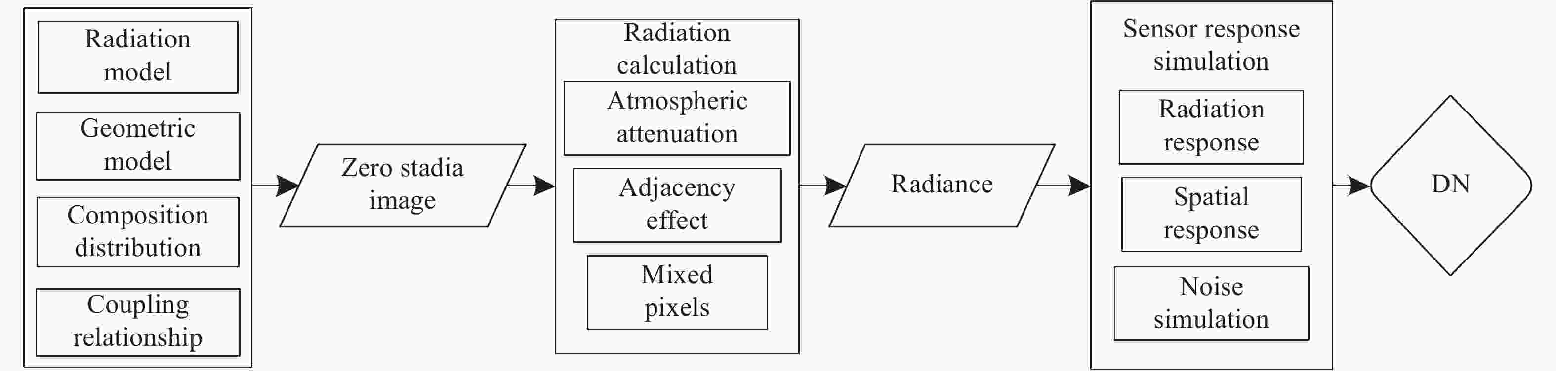
Figure 6.  High-resolution satellite ocean background imaging simulation flowchart

光学卫星传感器单个像元所能接收到的辐射能量可以表示为三部分辐射的总和，包括：（1）经过海表反射且未发生散射部分，L_su；（2）经海表反射后在大气中再次散射进入视场的部分，L_sd；（3）未到达海表，经大气散射直接进入传感器部分，L_sp。即传感器入瞳处接收到的所有辐射亮度可表示为：

式中：ρ(x,y,λ)表示地面反射率；λ表示波长；τ_v表示大气上行透过率；τ_s表示大气下行透过率；E⁰表示太阳到达大气层顶的辐照度；θ表示太阳天顶角；T(x,y)表周边像元对中心像元的辐射贡献比重，可用第1章中的三维海面辐射模型及蒙特卡罗模拟的周边像元邻近效应进行描述^[18-19]；E^d表示大气向下散射的辐照度。该部分各大气参数的数值，在确定观测条件后，都可根据成熟的辐射传输模型MODTRAN (MODerate resolution atmospheric TRANsmission)计算得到。

利用逆向蒙特卡罗光线跟踪方法^[20-21]，通过随机地向从传感器向观测场景发射成千上万条光线，跟踪它们与大气和场景的相互作用，并返回光线与场景碰撞点处的出射辐射亮度场，叠加上大气的衰减和程辐射作用后返回该点在入瞳处的辐射亮度。

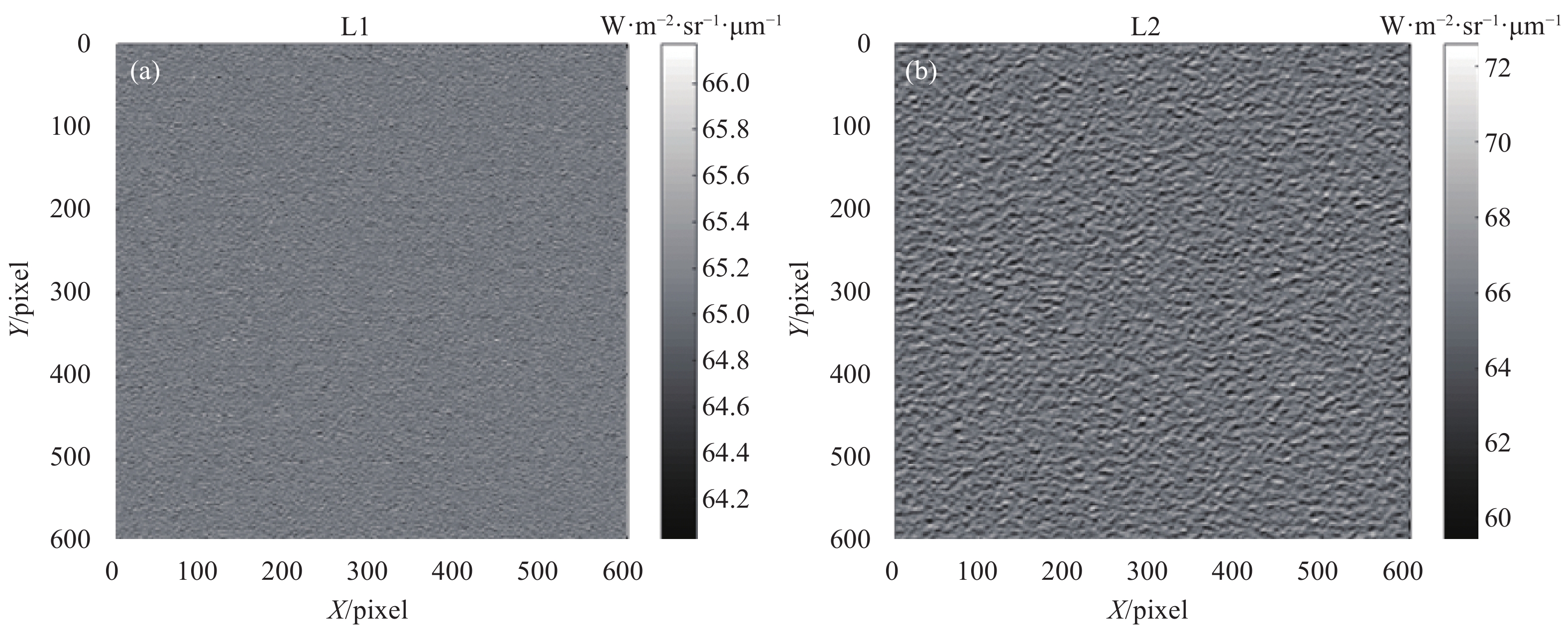
假定卫星垂直观测，大气条件良好的情况下，模拟计算分辨率为0.5 m，图像大小为600×600的海面图像，不同海浪等级下450~520 nm波段海面辐亮度在卫星入瞳处分布如图7所示。

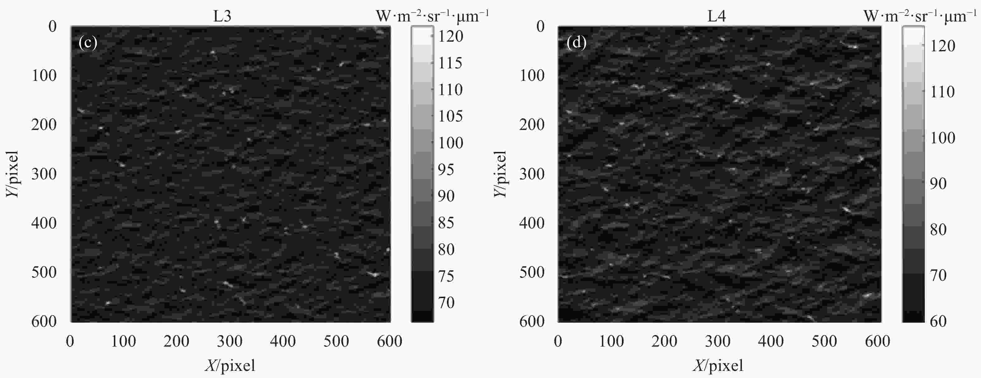
Figure 7.  Radiation field at the entrance pupil of the satellite under different wave levels. L1: Level 1 waves; L2: Level 2 waves; L3: Level 3 waves; L4: Level 4 waves

(1)传感器光谱响应模拟

从传感器孔径前段探测到的大气层顶辐亮度信号转化为探测器输出的光电信号DN值这一过程，可以表示为：

式中:R(λ)为传感器的光谱响应；K为辐射定标系数；L₀(λ)为大气层顶的辐亮度信息；DN_dark为传感器暗像元的光电响应值；τ₀(λ)为传感器光学系统的透过率，为减少测量带来的误差，这部分会在传感器辐射定标时直接黑盒处理，体现在定标的信号增益系数中。根据中国资源卫星中心官网提供的数据，仿真的目标载荷ZY3-02星的全色多光谱相机（PMS）载荷各通道光谱响应曲线如图8所示。

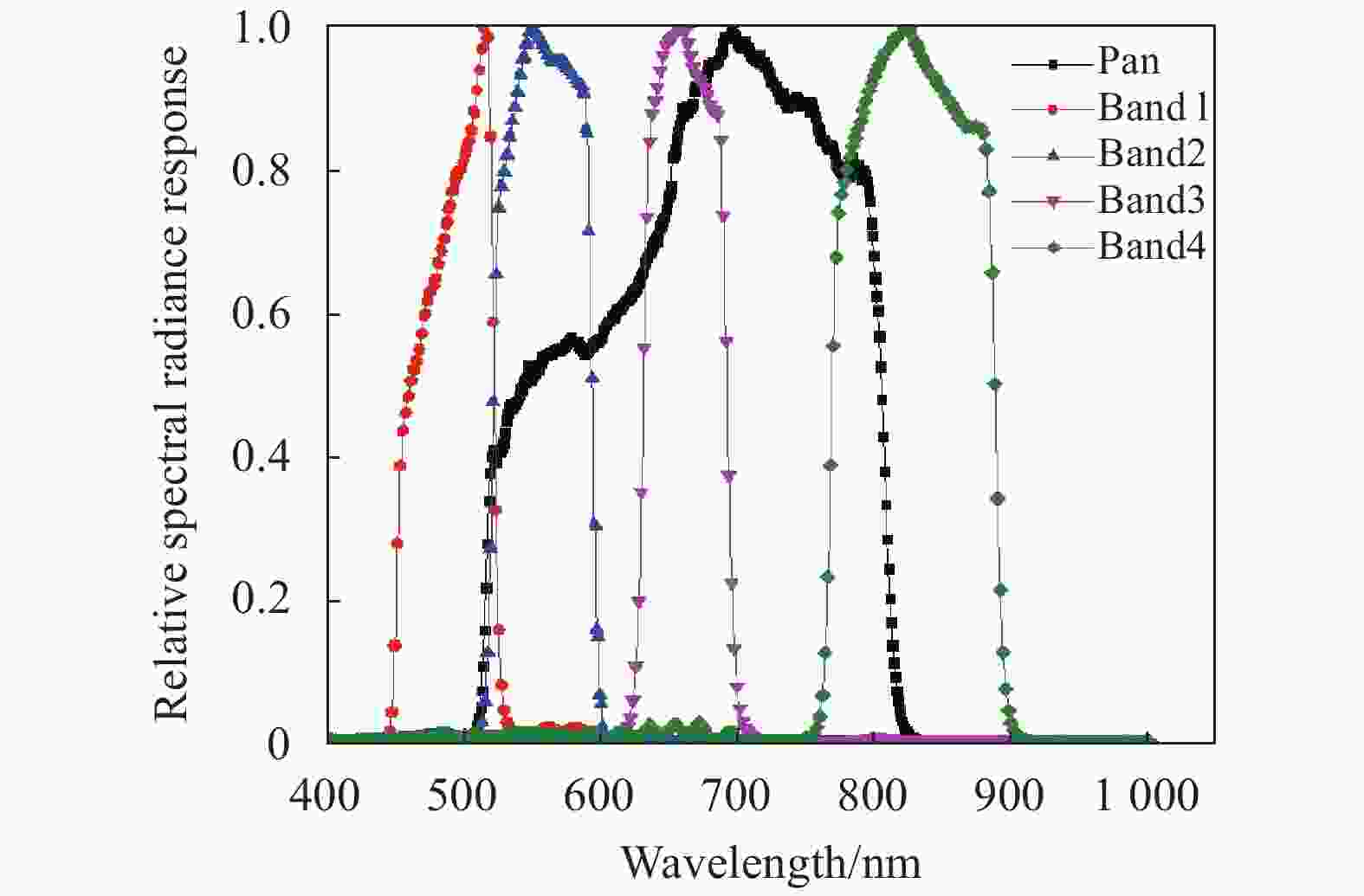
Figure 8.  ZY3-02 star PMS load spectral response function

(2)传感器空间响应模拟

在空间线性不变系统的假设下，可以采用空间频率域的MTF来描述传感器成像的空间响应，且总体响应的调制传递函数是各个环节MTF的乘积。

把传感器的响应看作是一个数学变换，经传感器光谱响应的图像表示为S{DN(x,y)}，(x,y)为参考平面的空间几何坐标，则传感器响应后的图像表示为：

式中：FT表示傅里叶变换；*表示卷积。因载荷的MTF多与传感器性能相关，其参数一般不对外公开。在这里利用目标卫星图像的明暗像元分界处，在对图像进行大气校正以后，采用刃边法计算相机的MTF^[22]。取卫星图像中的沿轨跟垂轨两个方向分别计算出相机Nyquist频率处的MTF值为0.073和0.186，取其均值约为0.13，作为相机的MTF。计算的点扩散函数及MTF曲线如图9所示。

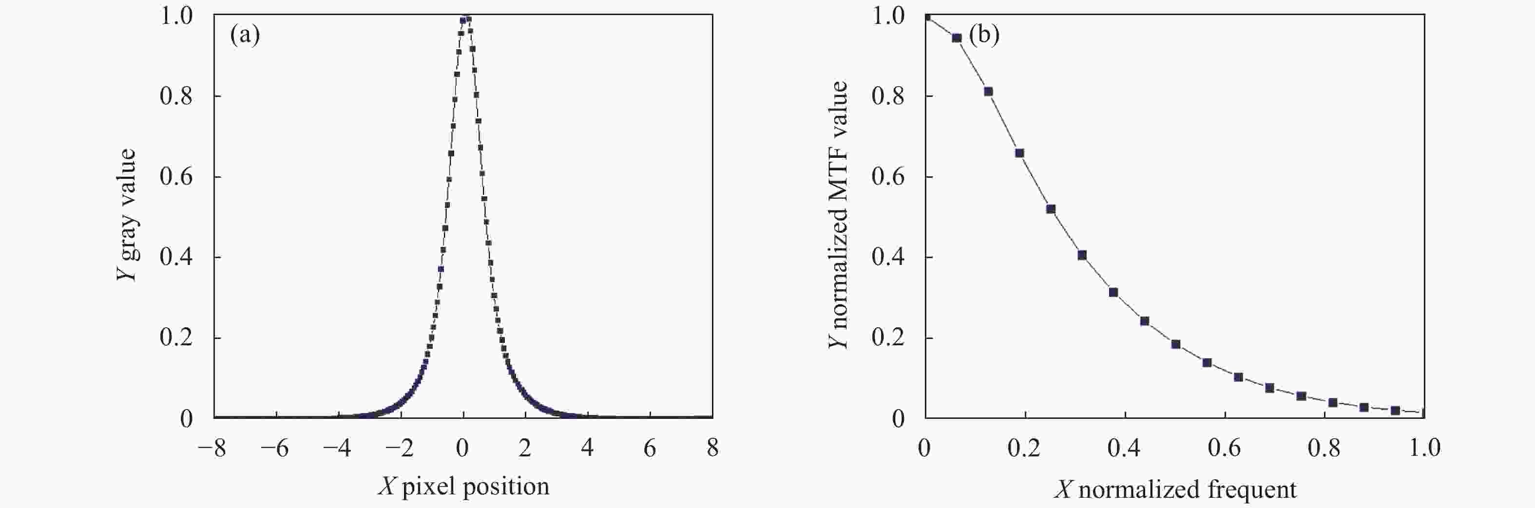
Figure 9.  Calculated camera point spread function and MTF curve. (a) Point spread function; (b) MTF

(3)噪声模拟

在上述信号的传输和转化过程中始终伴随着各种随机噪声的干扰，假设所有噪声都从传感器的输出端引入。对于CCD成像器件，占主导地位的随机噪声主要有背景光子散射噪声、暗电流散粒噪声、读出噪声和量化噪声。附加在输出信号上的全部随机噪声的总水平由他们各自统计分布的标准差决定。

文中采用的是白噪声模型，由均值为0，以传感器空间响应模拟后的图像标准差σ_N为标准差的Gauss随机数发生器产生，并表示成数字图像。

为了验证仿真结果的真实性，根据获取的ZY3-02星全色相机2019年2月7号拍摄的大连港数据，仿真模拟了在当时的大气及观测条件下的ZY3-02星多光谱相机卫星影像。仿真参数如表3所示。

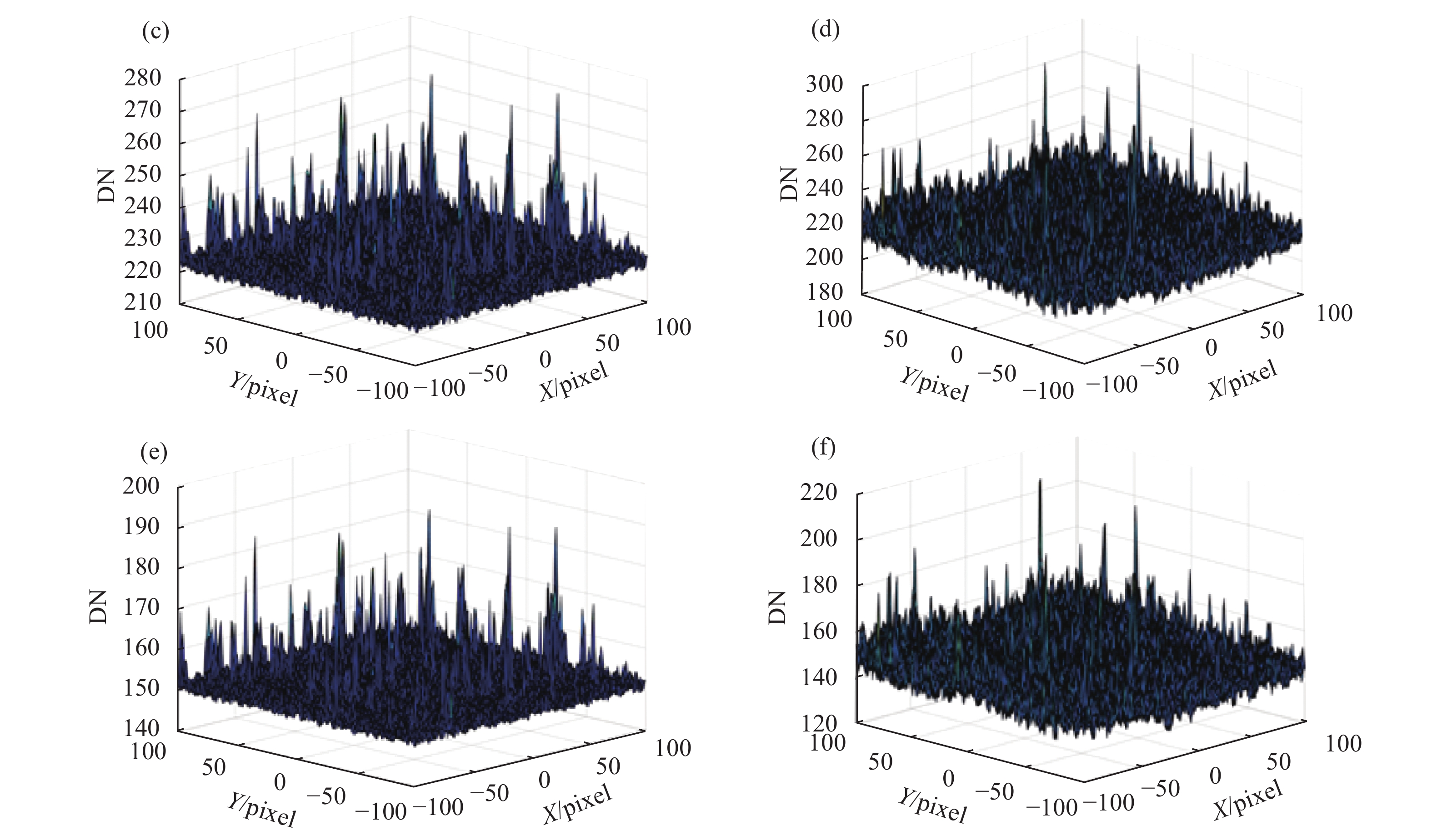
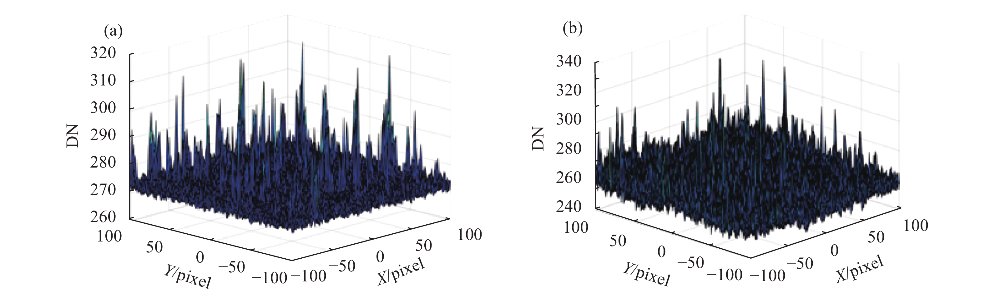
根据卫星成像时的风力等级选择对应的海浪模型进行仿真计算，得到4 000×4 000 pixel大小的仿真图像，为了更好呈现细节，截取200×200 pixel大小的海面图像及其DN值分布如图10、图11所示。仿真与卫星实测结果对比如表4所示。

Figure 10.  Comparison of simulation results with satellite data. (a) Simulating the sea surface of Band1; (b) ZY3-02 measured sea surface of Band1; (c) Simulating the sea surface of Band2; (d) ZY3-02 measured sea surface of Band2; (e) Simulating the sea surface of Band3; (f) ZY3-02 measuring the sea surface of Band3

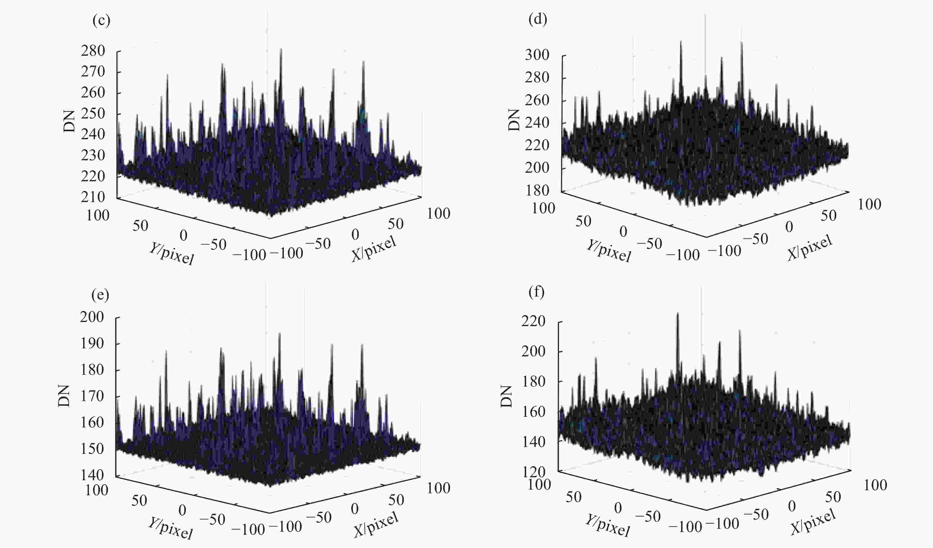
Figure 11.  Comparison of radiation distribution between simulated and measured results. (a) Simulating the sea surface of Band1; (b) ZY3-02 measured sea surface of Band1; (c) Simulating the sea surface of Band2; (d) ZY3-02 measured sea surface of Band2; (e) Simulating the sea surface of Band3; (f) ZY3-02 measuring the sea surface of Band3

通过仿真结果与卫星实测结果对比图，由图10可以看出，仿真的结果中，白帽的影响效果已经出现，海面的起伏状态也得到显示。但因卫星成像时刻，鉴于海上情况的复杂性与随机性，仿真的结果与卫星的实测结果在目视效果上存在差异。主要原因可能是构建的海面三维模型，是通过数学的方法模拟得到，而自然界的海浪受多种因素影响，单纯的数学模型无法完整的表征出其几何特征，且成像时刻海面的风场等影响模型构建的因素不一定均匀且稳定。

从图11仿真与实测结果辐射分布对比图以及表4的定量对比可以看出，仿真的结果与实测结果的相似度较高，其均值、极值相近，各波段的辐射强度相似，高值区域的离散分布情况相仿。这其中的误差则主要来源于辐射传输模型的计算及卫星辐射定标等系统误差。

文中综合考虑了高分辨率成像下海面呈现的波浪起伏、白帽、方向反射等细节因素，提出一种高分辨率海洋背景卫星成像仿真方法：将海面三维几何结构、组分分布和辐射特性结合，通过建立海面三维辐射场、大气和传感器效应模拟，得到卫星遥感仿真图像。与卫星实测图像比较，各波段仿真结果最大值误差8.6%，最小值误差7.8%，均值误差3.7%，标准差误差9.9%。在各波段平均灰度值、灰度分布、纹理细节等方面都具有较好的一致性。该方法将为进一步的高分辨率舰船目标仿真，以及目标与海面背景的耦合作用模拟提供必要基础。

该仿真方法在原理、模型和流程上基本正确，但一些输入参数因缺乏实际测量数据可能造成仿真结果存在一定误差。比如海水和白帽的方向反射模型，应当进一步通过实测反射率数据进行修正；海水的含盐量数据，Argo公布的是目标区域一个月份的平均值，并非卫星成像时刻的实测值；大气的光学厚度数据是MODIS准同步过顶数据的反演结果，并不是卫星过顶时的实测数据。这些在后续研究工作中，可以通过实测数据对模型做一定的修正，对误差源做进一步控制，得到更真实的仿真结果。