Solving initial structure of bifocal system according to theory of paraxial optics

变焦光学系统分为连续变焦和非连续变焦，连续变焦系统设计难度大，对机械结构要求高，其像面稳定性保证困难^[1]；非连续变焦主要以双焦、双视场光学系统为主，机械结构简单，容易装调且像面稳定^[2]。双视场既可以搭配使用，又可以单独使用，可满足不同的应用场合。利用短焦视场大的优点进行搜索、探测、观察；利用长焦测试精度高的优点来获取目标的详细信息，进行识别、确认和测量^[3-5]。在很多场合，双焦、双视场变焦系统可以替代连续变焦系统，应用于航空、航天、成像告警、搜索与跟踪等军事领域^[6-8]。

双焦、双视场光学系统比定焦光学系统设计难度大，其初始结构的选取也相对复杂，若通过光学设计软件直接设计出令人满意的双焦光学系统，其初始结构的确定十分重要^[9]。张葆等和晏蕾等通过三级像差理论求解双视场光学系统的初始结构，求解方法复杂、计算量大 ^[10-11]。尹骁等通过寻找专利进行缩放来求解初始结构，采用了七片透镜和两片非球面，该方法不具有通用性 ^[12]。

针对上述现状，需寻找一种通用、简便的方法来求解双焦、双视场光学系统初始结构。

双焦光学系统要求在变焦前后像面保持不变。其实现方法有两种：一是增加一个补偿组补偿焦面移动，该方法会增加机械结构的复杂性；二是在透镜移动前后遵循物像交换原则^[13-14]，保证物像共轭距不变，该方法机械结构简单。文中拟采用第二种设计方式实现。

采用物像交换原则设计双焦光学系统，按前固定组、变倍组和后固定组进行光学划分。其中：前固定组用于会聚无穷远物体的光线；变倍组用于改变焦距，达到变倍的目的；后固定组用于校正像差。

依据高斯提出的理想光学系统几何光学理论，研究近轴区成像规律建立理想光学系统成像模型，计算双焦光学系统光学结构的初始解。

图1给出了轴向双焦光学系统结构，当光学系统位于长焦时，${l_{2l}}$、${l'}\!\!_{2l}$为变倍组的物距和像距，d₂₃为后固定组和变倍组的间隔。当光学系统位于短焦时，${l_{2s}}$、${l'}\!\!_{2s}$为变倍组的物距和像距，d₁₂为变倍组和前固定组间隔。AA′为变倍组的共轭距。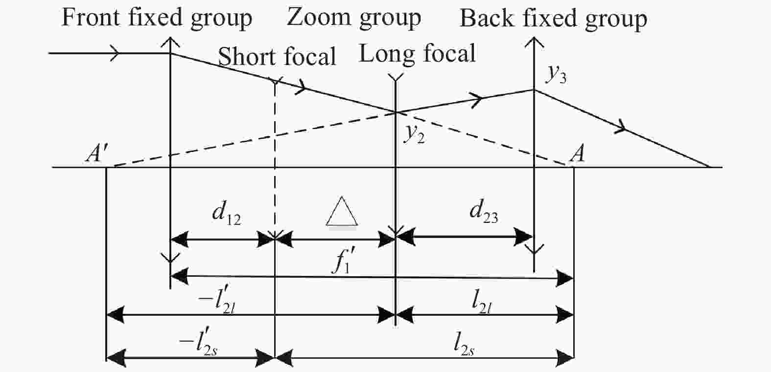

Figure 1.  Structure diagram of axial bifocal optical system

（1）变倍组相关参数计算

令变倍组焦距为$f_2'$，系统的放大倍率为$\beta $，则短焦和长焦时变倍组的垂轴放大倍率分别为：

由

可得短焦时变倍组的物距以及像距：

由物像交换原则可得长焦时变倍组的物距和像距：

当光学系统从短焦到长焦时，变倍组移动的距离为：

（2）前固定组焦距的计算

在对目标进行搜索和识别时，成像光学系统的物距可以认为是无穷远，则进入前固定组的光线是平行光入射且其光线的出射交点会聚于前固定组的焦平面上，该焦平面即为变倍组的物面。由此可以求出前固定组的焦距：

（3）后固定组焦距的计算

当光学系统位于短焦时，令系统的总光焦度为$\phi $，后固定组的光焦度为${\phi _3}$，前固定组和变倍组的等效组总光焦度为${\phi _{12}}$，等效组像方主平面与后固定组间隔为${d_{123}}$，则可以求出后固定组的焦距$f_3'$：

由于进入前固定组的光线为平行光，可得：

式中：$f_l'$为光学系统位于长焦时的焦距。

为了研究的方便性，针对一个具体问题进行设计分析，根据表1给出的具体设计指标要求，展开论述。

在双焦光学系统设计时，首先要确定变倍组焦距。由公式（8）可以看出变倍组的焦距决定了其移动范围，若焦距过大，则移动范围过大；若焦距过小，则其承担的光焦度过大，会引入较大像差导致公差敏感。其次要确定前固定组焦距，由公式（9）可以看出，前固定组焦距和${d_{12}}$有关，${d_{12}}$的选取主要考虑以下两个因素：一是系统的总长，二是主光线进入变倍组的入射高度和入射角度。由公式（9）、（12）可得，${d_{12}}$越大，${y_2}$越小，引入像差越少。最后确定后固定组的焦距，要考虑筒长以及与变倍组之间的距离${d_{23}}$，在不与变倍组相碰撞的前提下，由公式（13）可以看出，${d_{23}}$越小，${y_3}$越小，引入像差越小。此次设计共采用七片透镜，前固定组和变倍组各两片透镜，后固定组三片透镜。

根据上述选择分析，结合物像交换原则和高斯光学求解方法，得出各组焦距和间隔如下：$f_1' = 115 \;{\rm{mm}}$，$f_2' = {\rm{ - 35}}{\rm{mm}}$，$f_3' = 40\;{\rm{mm}}$，${d_{12}}$=20 mm，${d_{23}}$=10 mm。

首先将上述得到的焦距等数据输入ZEMAX中，将各组的间隔以及焦距大小设为变量，在评价函数中加入操作数EFFL控制焦距；再加入操作数ZTHI让长焦和短焦时总长相等，且前固定组和后固定组间隔相等，来保证焦距改变时变化的透镜组只有变倍组。另外，为保证像面稳定，需要在多重结构中将短焦时光学系统的后截距设为变量，长焦时光学系统的后截距设为拾取。进行优化即可得到图2所示的近轴光学系统光路图。优化后系统评价函数由0.000000038变为0，各组焦距和间隔分别为 $f_1' = 115.925\;{\rm{mm}}$,$f_2' = $$ {\rm{ - 35}}{\rm{.111}}{\rm{mm}}$, $f_3'{\rm{ = }}39.688\;{\rm{mm}}$，${d_{12}}{\rm{ = }}20\;{\rm{mm}}$，${d_{23}}{\rm{ = }}10.008\;{\rm{mm}}$。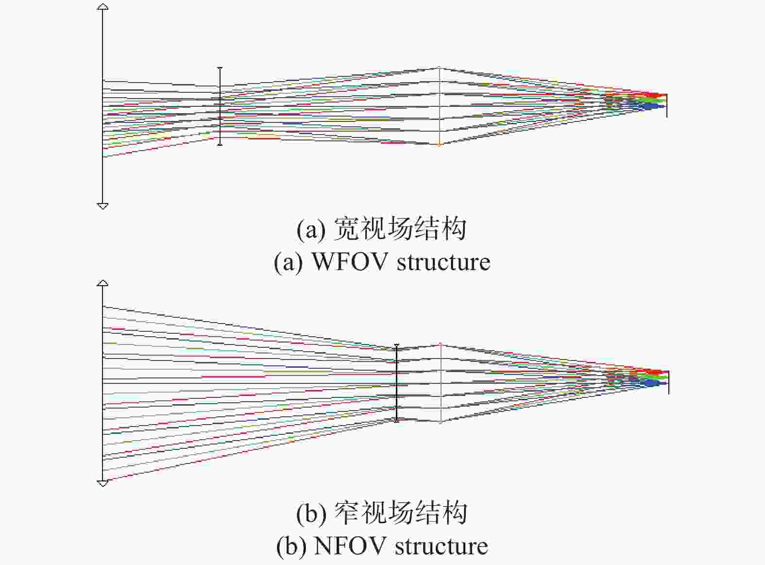

Figure 2.  Light path of paraxial optical system

近轴替代的核心思想是通过使用标准透镜来替代无像差的近轴面，进而再将标准透镜带入的像差优化到设计要求范围。

替换原则：第一步替换后固定组。采用透镜逐个插入法进行替代，在透镜插入系统时，要求其对系统的光焦度贡献为0，这一步的目的是使插入前后不改变任何光线轨迹。为了在不改变光学系统的情况下完成替代，需要逐步增加近轴面的焦距值，使近轴面的焦距接近无穷大，而插入的标准透镜组的焦距值接近近轴面最初的焦距值，然后删掉近轴面。在改变焦距的同时需要添加基本操作数控制球差、彗差等初级像差，并且需要控制透镜的厚度以及折射率，最后再将模型玻璃替换成真实玻璃。第一步的优化至关重要，若替换完后其像差过大，需要进一步优化，将RMS半径优化到6个像元以内，以便于后续替换过程能更好地平衡像差。第一步优化后光路图如图3所示，透镜参数如表2所示。

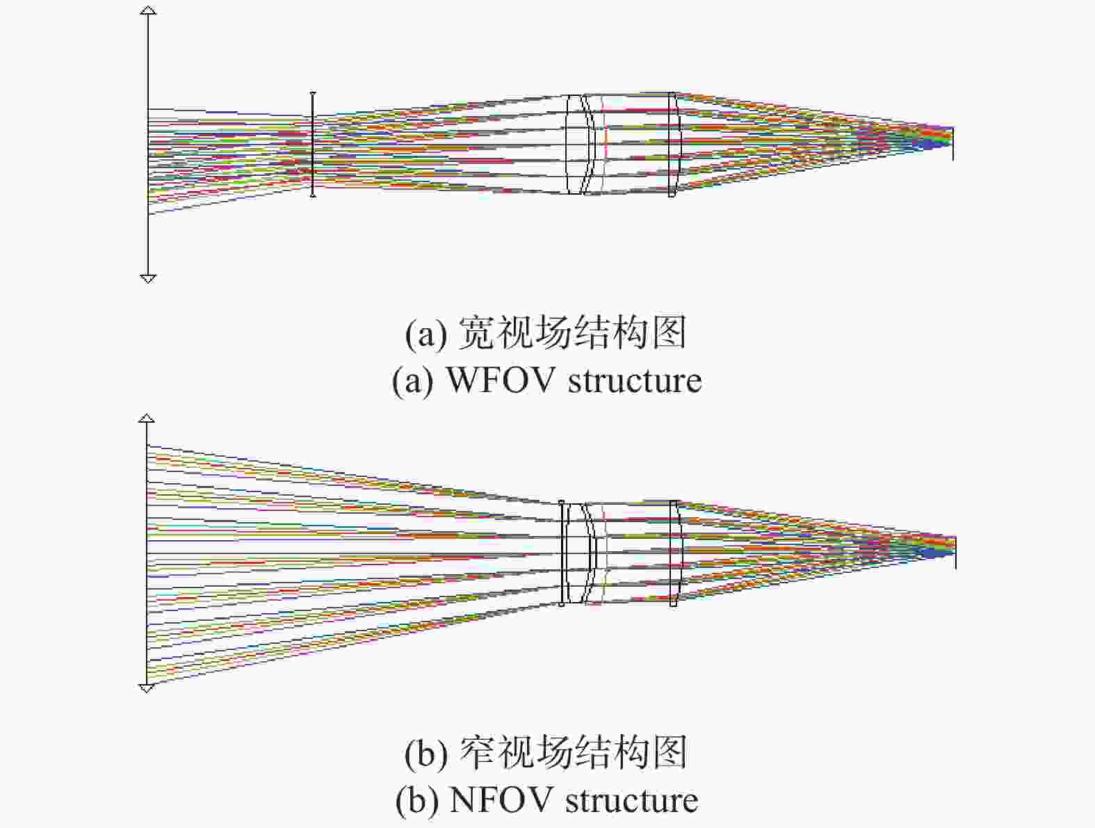
Figure 3.  Light path after the first step optimization

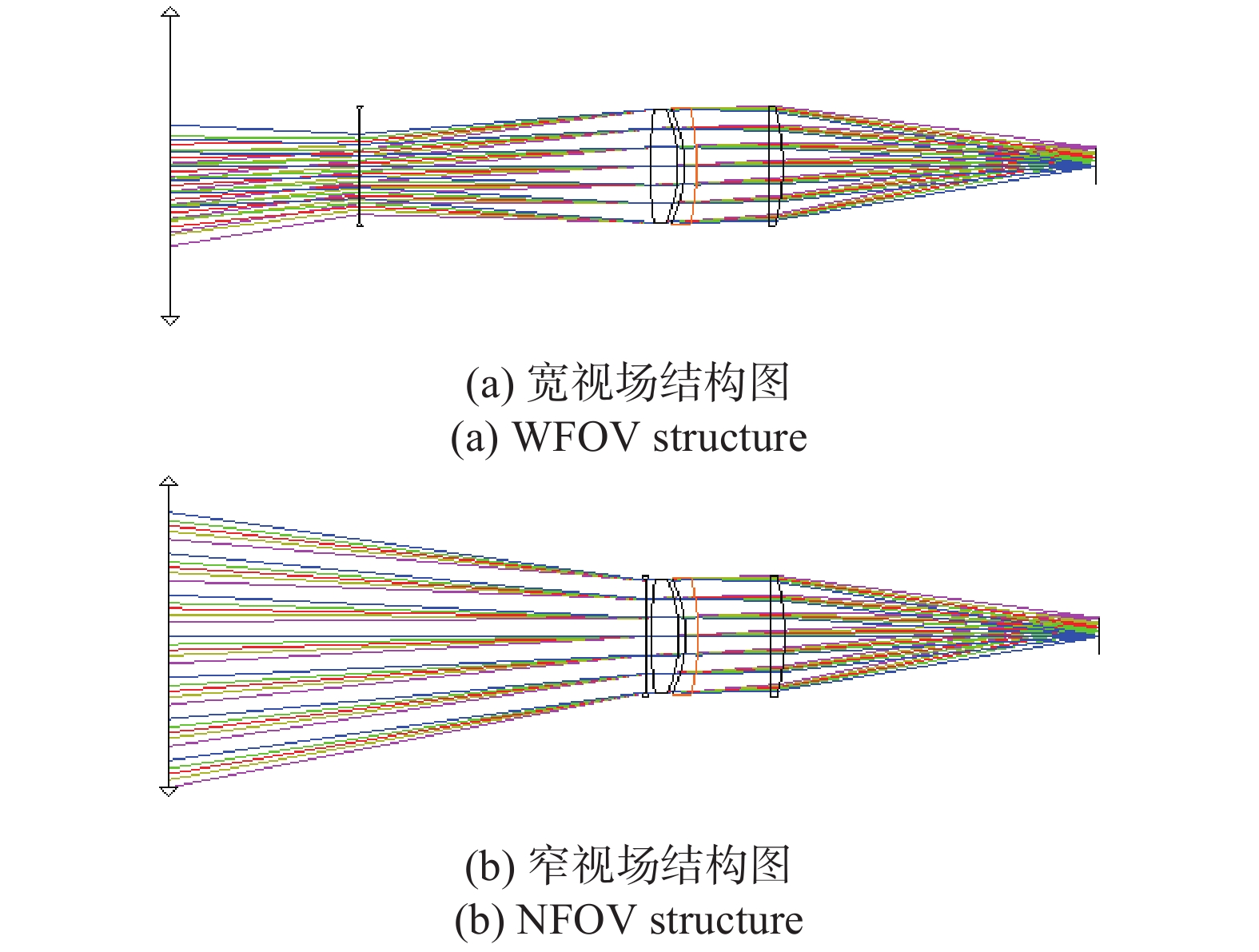
第二步替换掉变倍组。方法与第一步类似，逐步插入透镜，将近轴面的焦距逐步优化到无穷大，使加入的透镜焦距接近最开始近轴面的焦距，然后删掉近轴面，再次进行优化。第二步优化后光路图如图4所示，透镜参数如表3所示。

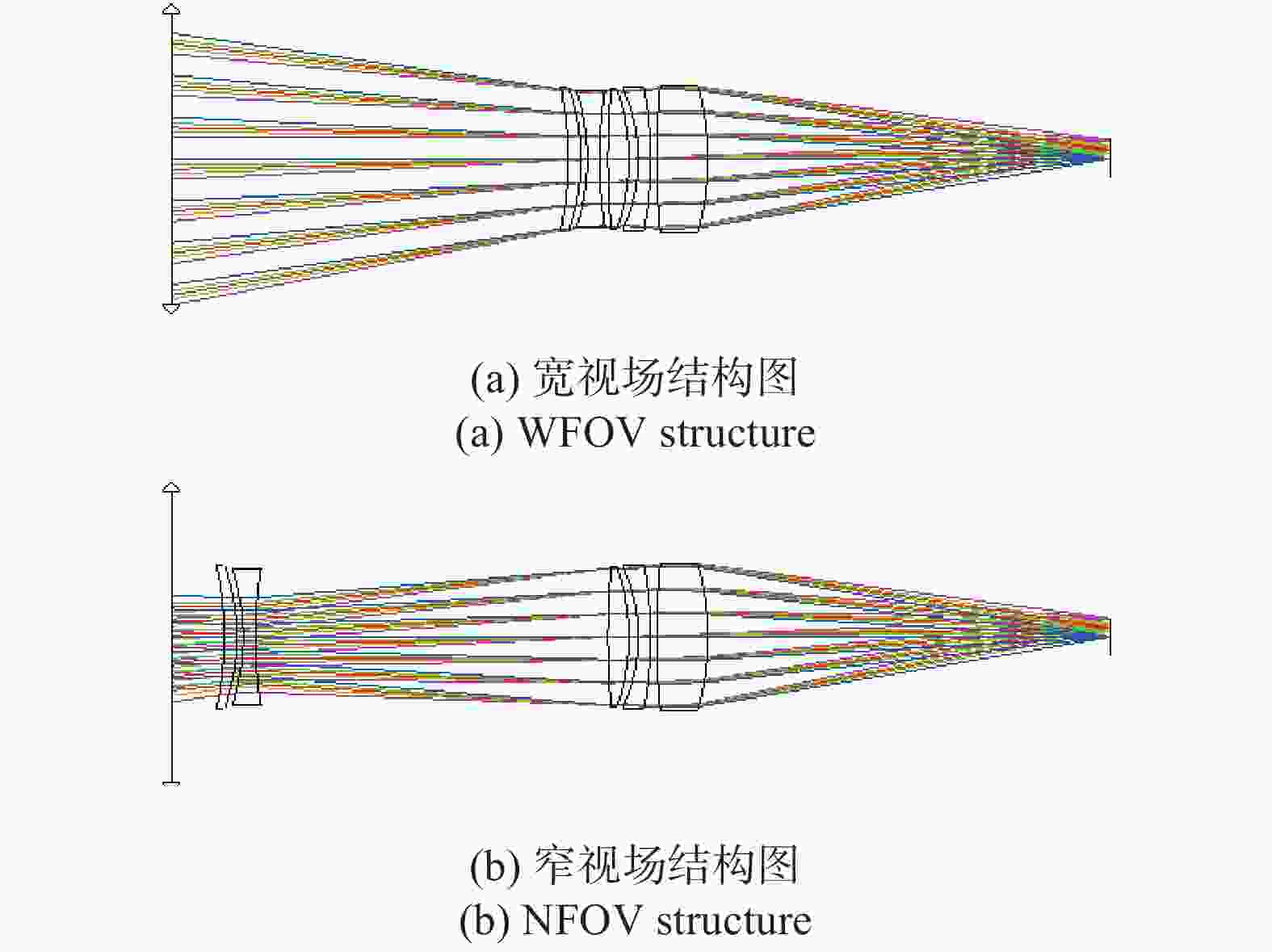
Figure 4.  Light path after the second step optimization

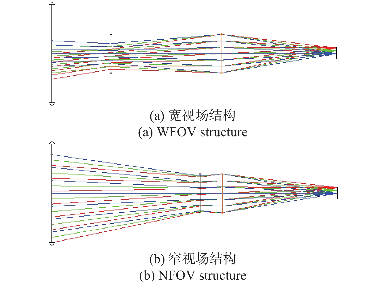
第三步替换掉前固定组。与第一步的步骤一样，应用相同的过程来替换近轴面，即得到的初始结构如图5所示。表4是第三步优化后透镜参数，表5是每一步优化后的像差大小。

Figure 5.  Light path diagram after the third step optimization

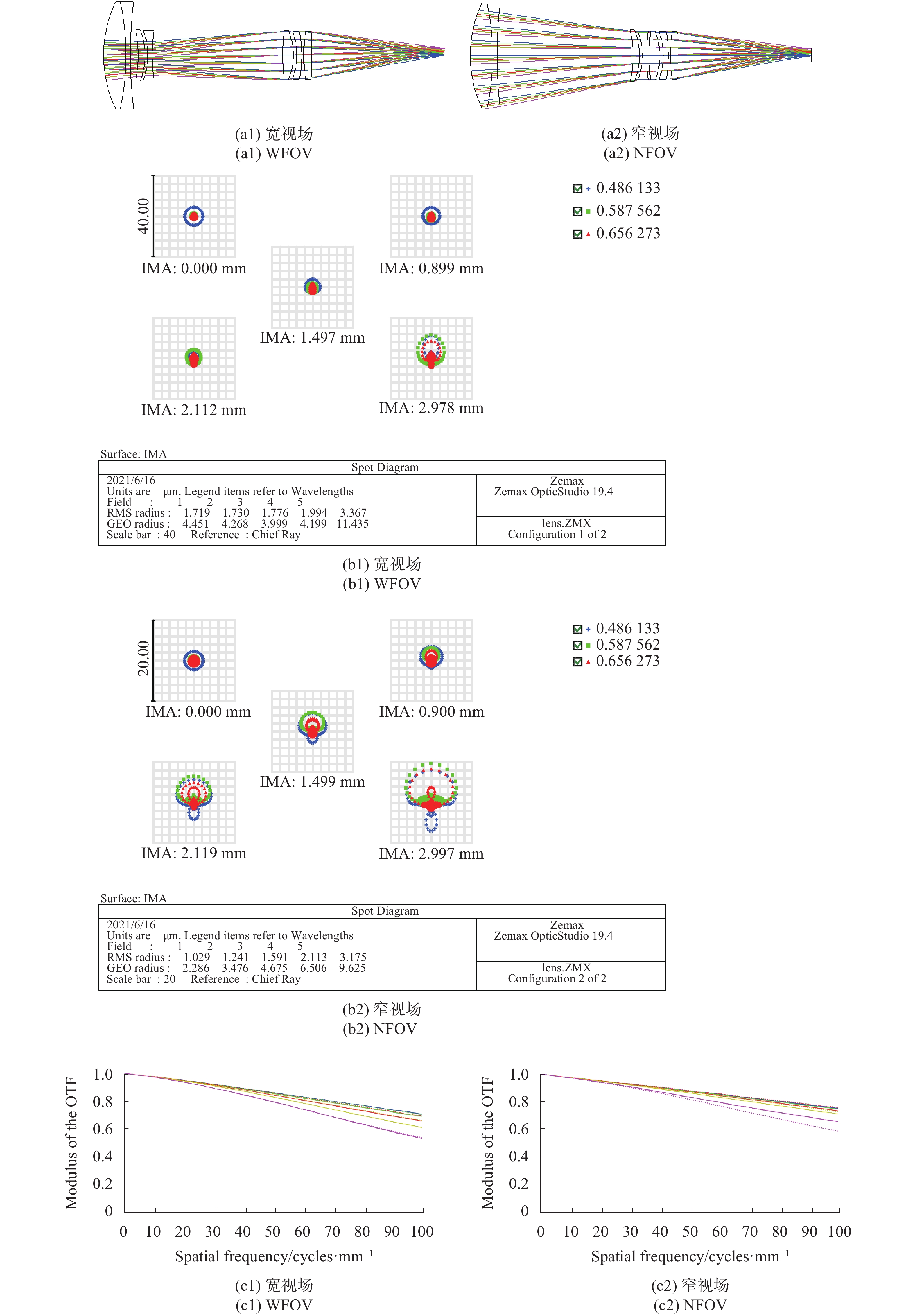
通过确定的初始结构按照像质要求对其进行进一步优化，并将初始结构中不常用的玻璃进行替换，优化后的系统光路和像差如图6所示。在0-0.707带视场处点列图皆小于0.5个像元大小，全视场处点列图小于0.7个像元大小；在宽视场时MTF大于0.52，接近衍射极限，场曲最大为0.0268 mm，畸变最大为0.7242%，垂轴色差最大为0.3 μm；在窄视场时MTF大于0.58，接近衍射极限，场曲最大为0.0289 mm，畸变最大为0.0527%，垂轴色差最大为2.7 μm。故该设计满足设计要求。

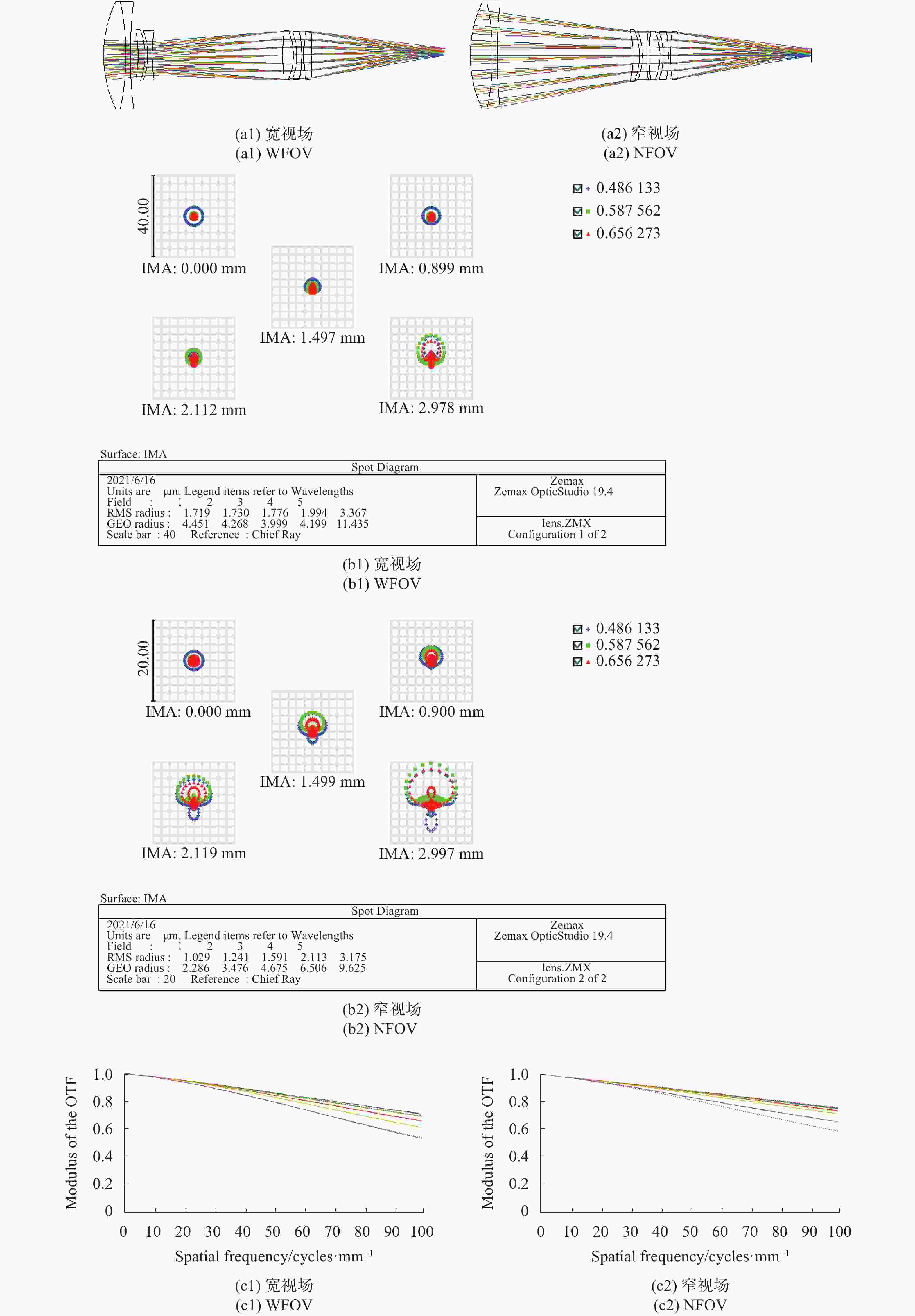
Figure 6.  Light path and aberration diagram. (a) Light path; (b) Spot diagram; (c) MTF; (d) Field curvature and distortion; (e) Lateral color

通过分析目前确定双焦光学系统初始结构方法的缺点，文中采用实际透镜分步替代各组分的近轴元件来获取初始结构，该方法的优点是将透镜的初始位置确定即可利用光学设计软件快速设计出双焦光学系统。在近轴区，光学系统成理想像，通过将实际透镜引入光学系统并将带入的像差进行平衡，得到一个新的初始结构，再进行优化得出符合要求的设计结果。

采用该方法在未使用特殊面型的情况下，用七片透镜设计出满足要求的结果，证明了该方法的有效性。从像质分析可以看出，该系统满足使用要求，可降低加工难度，节约成本，对装调和系统可靠性提供了保障。为光学设计中确定双焦、双视场初始结构提供了一个新方法。由于任何实际光学系统都可以看做是一个理想光学系统转换成有像差的光学系统，故该方法具有普适性。