Beam deflection correction model of wedge-shaped shock waves over hypersonic vehicles

Hypersonic vehicles can complete specific tasks while traveling at hypersonic speeds (at Mach numbers of 5 or above)^[1]. Long gliding flights are possible in near space (at 20–100 km). These vehicles are expected to be deployed widely in the future^{[2, 3]} owing their ability to fly at high speeds, respond rapidly in combat situations, cause significant damages, strong maneuvering, and penetrate effectively^[4-5]. However, the reliability of hypersonic vehicles is limited due to the lack of effective autonomous navigation methods, which are required for functions such as high-speed cruising, high-load maneuvers, and penetration, along with encountering highly intense confrontational situations^[6].

Celestial navigation is an autonomous navigation method that utilizes star sensors to detect celestial bodies and obtain star maps from which navigation information, including positions, speeds, and attitudes of carriers, can be acquired^[7]. Hence, celestial navigation is based on optical observations of star tracker sensors. However, because hypersonic vehicles travel at high Mach numbers in near space, the data collected by optical sensors are influenced by factors such as shock waves outside the vehicles and turbulence fields near the windows^[8-9]. Consequently, the imaging targets tend to be distorted and blurred, while jittering and energy attenuation can occur. These aero-optical effects directly influence star map acquisition and celestial navigation solutions^[10-12]. Therefore, to promote the application of celestial navigation in hypersonic vehicles, the effects of shock waves on beam deflection must be understood and corrected.

The occurrence of shock waves over hypersonic vehicles is inevitable. Research has shown that small and large shock wave structures form at a convective Mach numbers above 0.7 and 1.2, respectively^[13]. Furthermore, most hypersonic vehicles in the United States and Russia have waverider designs ^[14]. Therefore, the heads of the vehicles have sharp wedges, which induce full shock wave’s structure^[15-16]. Higher Mach numbers result in stronger effects of the shock waves^[17]. For example, the cross-sections of the main bodies of X-43A and X-51A (developed in the United States) are wedge-shaped. Thus, the effects of wedge-shaped shock waves must be considered during the collection and calibration of star maps for navigation.

One important property of a shock wave is that it can create a curved surface with almost zero thickness and cause dramatic state changes in a continuous medium. In addition, it causes the physical properties (e.g., density, speed, pressure, and temperature) of the media in front of and behind the curved surface to differ considerably^[18]. Thus, it causes the deflection of starlight.

Early-stage research on shock wave structures was based on infinitely long flat plates. Many studies were based on the assumption that the carrier in the high-speed flow field is an infinitely long flat plate with a sharp leading edge. Kendall provided a rapid method to calculate the slopes of the shock wave surfaces using this assumption^[19]. Garvine studied shock wave propagation models^[20], and Butler proposed a method for conducting numerical simulations involving infinitely long plates^[21]. Yin et al. classified shock waves caused by pointed and blunt bodies and established a basic model of beam deflection due to shock waves^[22]. The stability of the hypersonic shock layer (velocity, temperature, density, and pressure) had been calculated^[23]. Nevertheless, these studies did not address problems such as the propagation of measurement errors. Subsequent research in China focused on shock wave structures around conical bodies and their effects^[24]. Nevertheless, there are few studies on beam deflection due to wedge-shaped shock waves and the resulting error propagation. That would be the key to control the error of real-time deflection correction.

This paper examined an analytical algorithm for the modeling of wedge-shaped shock waves based on aero-optical theories (Section 1). Next, an ideal beam deflection model and a shock wave measurement error propagation model were established. A quantitative correction model of beam deflection due to shock waves over hypersonic vehicles was constructed (Section 2). The relation between the Mach number and shock wave angles and density variations were calculated. Based on the simulation results, the shock wave angle measurement errors propagation model and their effects on beam deflection were analyzed and confirmed (Section 3). A reference basis for extending the starlight navigation to the hypersonic vehicle can be afforded.

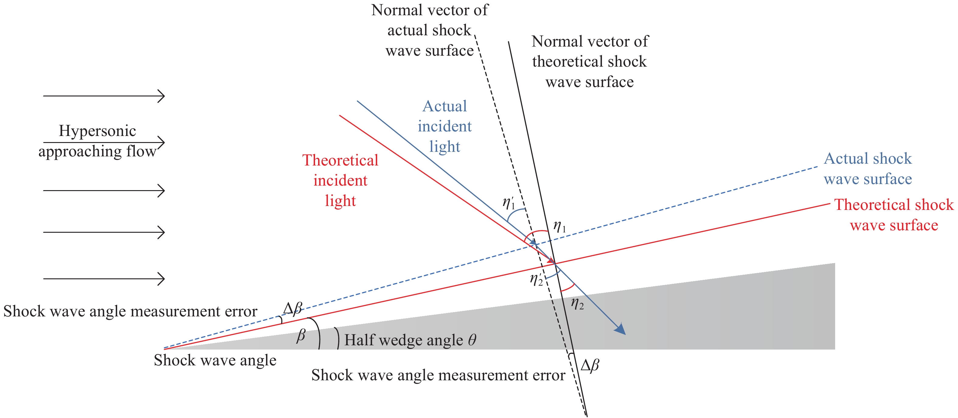
By denoting the half wedge angle of the wedge as $\theta $ and the shock wave angle as $\;\beta $(Fig.1), the density of hypersonic approaching flow above and under the shock wave surface as $\;{\rho _1}$ and $\;{\rho _2}$ respectively, the key parameters $\;\beta $ and ${{{\;\rho _2}} / {{\rho _1}}}$ can be calculated as follows^[25]: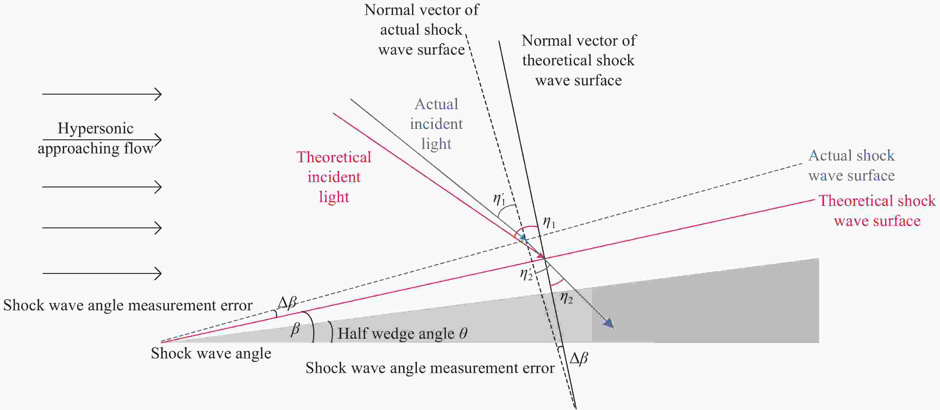

Figure 1.  Schematic of wedge-shaped shock waves and beam deflection

where, ${M_1}$ is the Mach number of the approaching flow and $K$ is a constant. In this section, an analytical algorithm model is presented to solve the wedge shock angle derived from Eq. (1).

When $\zeta = \cot \;\beta $ and ${\sin ^2}\;\beta = \dfrac{1}{{1 + {\zeta ^2}}}$, Eq. (1) can be converted into a linear expression as follows:

The post-wave Mach numbers of hypersonic wedge shock waves are greater than 1. Therefore, given a known Mach number of the inlet flow, ${M_1}$, and a known half wedge angle, $\theta $, the above cubic equation with one unknown $\zeta $ can be solved analytically^[26] as follows:

In Eq. (4), the parameter $p$ and $q$ can be expressed as follows:

And a discriminant $\Delta = {(q/2)^2} + {(p/3)^3}$ can be obtained. When $\Delta < 0$, there are three distinct real roots. When $\Delta = 0$, there is a double real root. Finally, when $\Delta > 0$, one real root and two complex conjugate roots are obtained. Additionally, if $\Delta < 0$, the shock waves are attached. The shock wave angle, $\;\beta $, could be calculated with the results of Eq. (4) as follows:

If the air density of hypersonic approaching flow above the shock wave surface, $\;{\rho _1}$, is known, then Eq. (2) can be used to determine the air density under the shock wave surface $\;{\rho _2}$.

According to the Lorenz–Lorentz equation, the relationship between the density of the medium in the flow field, $\rho $, and the optical refractive index, $n$, can be written as follows:

For gaseous media, $n \approx 1$, Eq. (6) can be simplified to represent the relationship between the refractive index and the medium density as follows:

In Eq. (7), ${K_{GD}}$ is the Gladstone–Dale constant, which can be approximated as a function of wavelength using the following empirical equation^[27]:

For angles of incidence and refraction ${\eta _1}$ and ${\eta _2}$, Snell's law states that $\dfrac{{\sin {\eta _1}}}{{\sin {\eta _2}}} = \dfrac{{{n_2}}}{{{n_1}}} = \dfrac{{1 + {K_{GD}}{\rho _2}}}{{1 + {K_{GD}}{\rho _1}}}$, respectively. Hence, the angle of refraction after light travels through shock waves, ${\eta _2}$, can be calculated by the star trackers. And the incidence beam angle, ${\eta _1}$, is as follows:

Owing to the compression effects of shock waves, we can know ${\rho _2} > {\rho _1}$. Thus, the deflection angle of light, $\Delta \eta $ can be given as follows:

The structure of the hypersonic shock wave can only be accurately obtained under a good experimental environment. Therefore, the analytical value of the shock wave angle, $\;\;\beta $, which was mentioned in 3.1, can be used to replace the actual measured value for calculation processing. The difference between the analytical value and the true value is recorded as measurement error $\Delta \;\beta $. And the actual shock wave angle, $\;\;\beta '$, is given as follows:

In actual observation, the vector of emergent beam can be measured by the star sensor. But the definition of the incident and the refraction angle, ${\eta _1}$ and ${\eta _2}$, as well as the determination of the density behind the shock surface, ${\;\rho _2}$, all depend on the shock angle. The refraction angle determined by the analytical shock wave angle $\;\beta $ is denoted as ${\eta _2}$. The actual angle of emergent beam, ${\eta '_2}$, becomes:

According to Eq. (2), the actual density of the gas behind the shock wave surface, ${\rho '_2}$, and the actual angle of incident, ${\eta '_1}$, can also be written as follows:

By using $Q' = \dfrac{{1 + {K_{GD}}{{\rho '}_2}}}{{1 + {K_{GD}}{\rho _1}}},Q = \dfrac{{1 + {K_{GD}}{\rho _2}}}{{1 + {K_{GD}}{\rho _1}}}$, we obtain:

Therefore, the correction error factor caused by $\Delta \;\beta $, can be expressed as:

${\eta '_1},{\eta _1}$ can be expanded with follow formulas:

$\Delta \;\beta $ is in radians and its value is as small as ${10^{ - 2}}$, so we can assume that $Q' \approx Q \approx 1$ and the expansion has to be accurate up to ${(\Delta \;\beta )^2}$. This hypothesis will be verified in Section 3. Thus, we obtain:

Similarly, because $Q' \approx Q \to 1$, $({Q^3} - Q)/2 \to 0$. When the angle of incidence, ${\eta _1}$, is relatively small as ${10^{ - 1}}$, the following approximations can be made:

Finally, a simplified error propagation equation was obtained:

We termed Eq. (19) as "the rapid calculation model of error propagation". Based on this model, when $\Delta \;\beta $ and ${\eta _2}$, are small enough, the effects of $\Delta \;\beta $ on the deflection angle of light are almost linear.

As mentioned above, the direction of the refracted star light could be calculated by the star sensor. It could be used with the actual shock wave angle $\;\beta '$ to achieve ${\eta '_2}$. What we actually want is the original incident angle of the starlight, ${\eta '_1}$. Since the hypersonic shock wave of the aircraft cannot be accurately measured in real time, ${\eta '_1}$ can be represented by the theoretical analytical value, ${\eta _1}$, with the correction error factor, $\Delta {\eta _{\Delta \;\beta }}$.

The quantitative correction model of beam deflection due to shock waves over hypersonic vehicles can be constructed as follow:

If Eq. (20) was used to describe the beam deflection of the hypersonic shock wave, the beam error after the correction would be $\Delta \;\beta + {{10\eta _2^3{{(\Delta \;\beta )}^2}} / 3}$.

The navigation modules are located on the slopes of the wedges (Fig.2). Based on the assumptions on simplifying the side section of waverider hypersonic vehicle to a wedge structure in Section 1, the half wedge angle $\theta $ could be set as 0.1359 radians. Different wedge angle values ​​can be assigned for the other waverider wedge structures.

Figure 2.  Load layout^[28] and wedge-shaped structure of preliminary vehicle

Furthermore, the following parameters were used in the simulations: the altitude of the vehicle as 20 km, specific heat ratio of the gas $K = 1.41$, medium density of the approaching flow in the flight area ${\;\rho _1} = 0.088\;91\;{\rm{kg}}/{{\rm{m}}^3}$; angle of attack angle is 0°; atmospheric pressure of 5529.3 Pa; air temperature of 216.65 K.

Using Eq. (9) and Eq. (10), the shock wave angle, $\;\beta $, and the ratio of the density of the media above and under the shock wave surface, $\;{\rho _2}/\;{\rho _1}$, at different Mach numbers ($Ma = 5.0,5.5,6.0,6.5,7.0,7.5,8.0$) were calculated. The results are summarized in Table 1.

The beam deflection angle, $\Delta \eta $, when light traveled through shock waves at different angles of incidence ($10^\circ ,20^\circ ,30^\circ ,40^\circ ,50^\circ $) were also obtained in Table 2. The angle is generally measured in degrees or radians in design and manufacture of aircrafts or sensors. In the process of celestial observations, the angle of beam deflection is usually measured with arcseconds. Therefore, arcsecond was used as the unit of beam measurement in the tables and figures below.

As can be seen in Table 1, as the Mach number increases, the compression effect of the shock waves and the density ratio increase and the shock wave angle reduces gradually. The results reported in Table 2 and Fig.3 reveal that beam deflection becomes more significant as the Mach number and angle of incidence increase. At Mach numbers of 5-8, the deflection angles can be up to 6.8".

Airborne celestial attitude determination systems could provide an attitude solution with accuracy better than 1.0" RMS^[29]. And the beam deflection was needed to be corrected to achieve such accurate for observation.

Figure 3.  Deflection angles due to shock wave surfaces at different Mach numbers and angles of incidence

Under hypersonic conditions, the experimental observation of shock wave structure is very difficult. The researches on the shock wave of hypersonic vehicle were mainly carried out with computational fluid dynamics (CFD) technology, which did not rely on simplified physical models, but used numerical algorithms with the help of computers to directly solve fluid flow functions. However, CFD processing requires huge computing resources, and the real-time performance is not good enough^[30].

The shock wave structure and the light deflection caused by it could be calculated by analytical methods as Section 2. If the CFD solutions were used as the actual results, the error analysis of the theoretical results could be carried out to improve the accuracy of the theoretical analytical model.

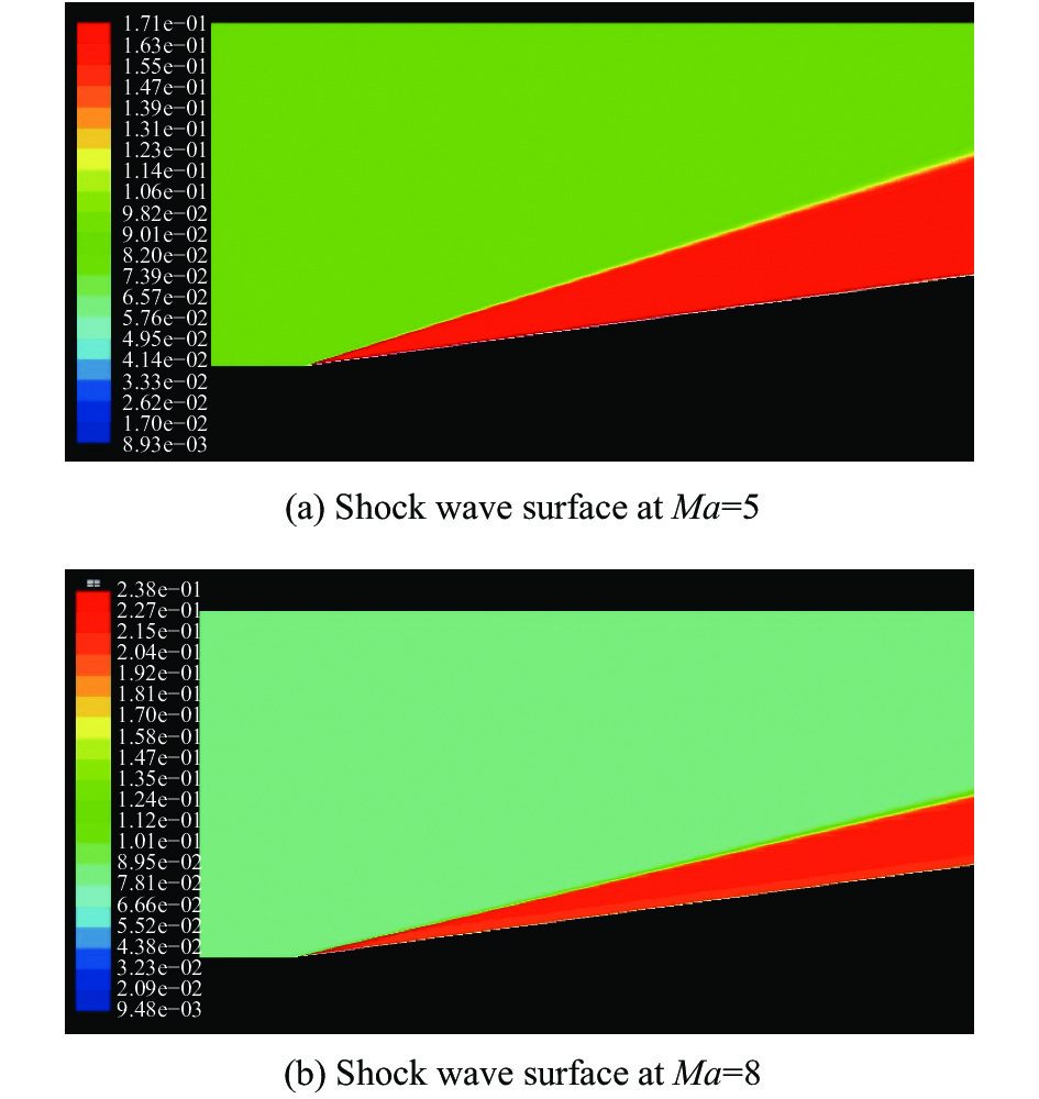
The deviations of the theoretically calculated shock wave angles from the actual values will cause the deflection angles to vary. Therefore, CFD simulations at Mach numbers of 5–8 were performed using the defined parameter values. The results demonstrated that stable shock wave structures formed over the wedge under all the aforementioned conditions (Fig. 4). However, the measured shock wave angles obtained through CFD simulations differed from the theoretically calculated ones.

Figure 4.  CFD results of wedge shock waves at different Mach numbers

The measured shock wave angles were extracted from the CFD raster data. Table 3 presents the deviations of the simulated shock wave angles from the theoretical values at different Mach numbers.

Under the same conditions, the measurement error, $\Delta \;\beta $, does not increase as the Mach number increases. Hence, further investigations are required to determine whether the simulation errors are random.

According to the conclusion given in Section 4, when the measurement errors, $\Delta \;\beta $, and the angle of incidence, ${\eta _1}$, are smaller than ${10^{ - 1}}$, $\Delta \;\beta $ has a negative and linear relation with the deflection angle.

However, this is based on the assumption that $Q' \approx Q$; $Q'$ and $Q$ were solved separately at different $\Delta \;\beta $ values from 0° to 5.0° at $Ma = 3,5,8$. The similarity between $Q'$ and $Q$ was determined using $\left| {(Q' - Q)/Q} \right|$, and the results are presented in Table 4.

From the table, it can be seen that the values of $\left| {(Q' - Q)/Q} \right|$ are in the order of ${10^{ - 4}}$ under all conditions. Therefore, the assumption that $Q' \approx Q$ stated in Section 3 is valid.

The shock wave structure and the light deflection caused by it could be calculated by analytical methods as Section 2. If the CFD solutions were used as the actual results, the error analysis of the theoretical results could be carried out to improve the accuracy of the theoretical analytical model.

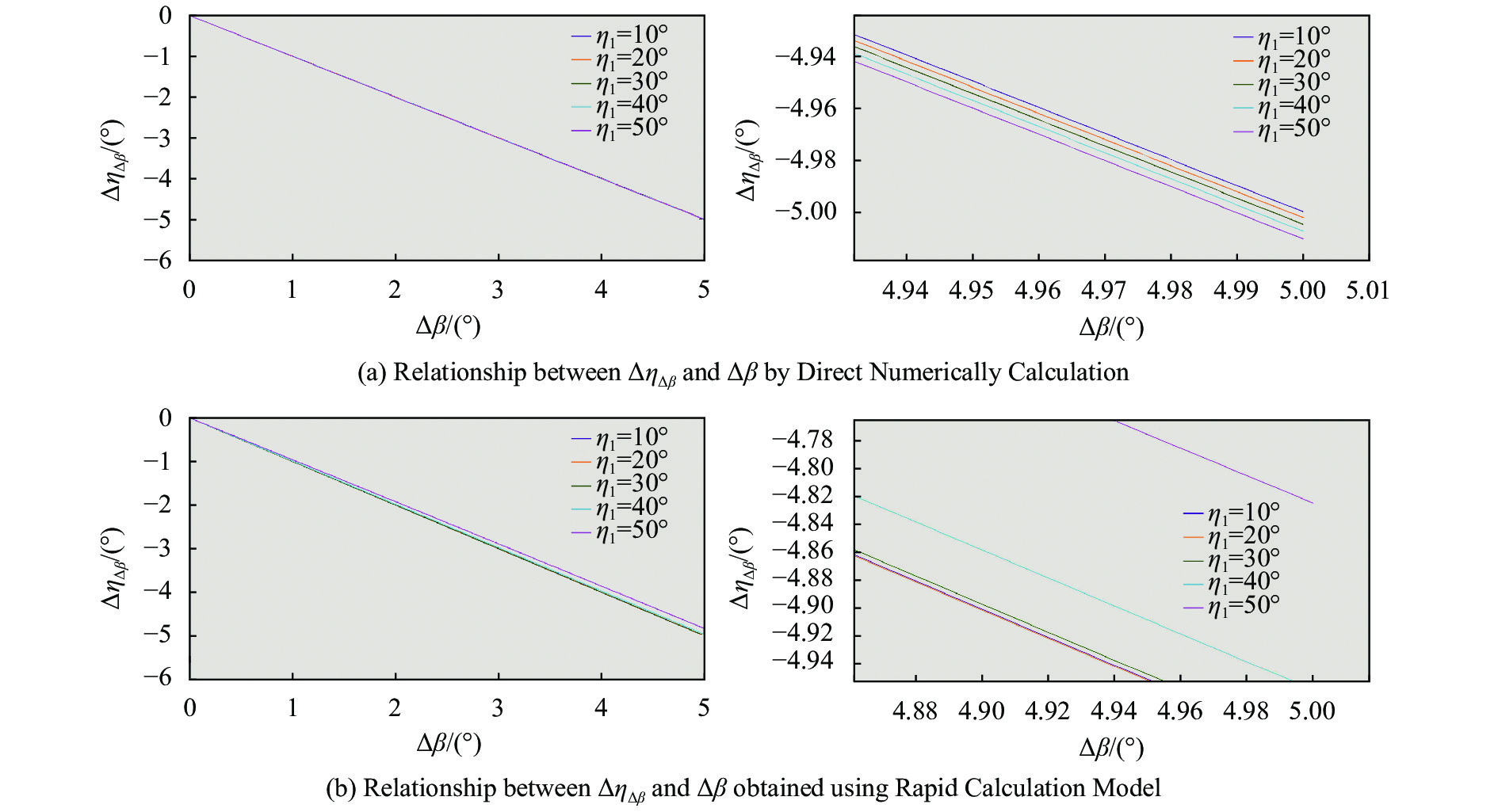
In the range of $\Delta \;\beta $ considered in this study, the error propagation, $\Delta {\eta _{\Delta \;\beta }}$, can be calculated in different ways. Direct Numerically Calculation can be performed using Eq. (6), and Rapid Calculation Model from Eq. (19) can be used for rapid approximation results.

From the figures below, it can be seen that $\Delta {\eta _{\Delta \;\beta }}$ and $\Delta \;\beta $ generally have a negative linear relationship. When the angle of incidence is smaller than $50^\circ $, the errors estimated via rapid approximation and direct numerical calculation are similar. However, as the angle of incidence, ${\eta _1}$, increases, ${c_1} = \left(\dfrac{Q}{2} - \dfrac{{{Q^3}}}{2}\right)\eta _1^2 + \dfrac{{5{Q^3}}}{{18}}\eta _1^4 - Q$ in Eq. (17) could no longer be approximated to $ - Q$. Therefore, the results obtained using Rapid Calculation Model started to deviate from those obtained through the Direct Numerically Calculation.

If an equation similar to $\Delta {\eta _{\Delta \;\beta }} \approx c + {c_1}\Delta \;\beta + {c_2}{(\Delta \;\beta )^2}$ in Eq. (17) is used to fit the relationship between $\Delta {\eta _{\Delta \;\beta }}$ and $\Delta \;\beta $ at a certain angle of incidence ${\eta _1}$, as shown in Fig.5(a), then the above expression becomes $\Delta \eta = a + {a_1}\Delta \;\beta + {a_2}{(\Delta \;\beta )^2}$. Figure 6 shows the differences between the curve parameters used for the Direct Numerically Calculation solutions ($a,{a_1},{a_2}$) and those used Rapid Calculation Model ($c,{c_1},{c_2}$) for different ${\eta _1}$.

Figure 5.  Linear relationships between deflection angles and shock wave

Figure 6.  Comparison of parameters used in numerical calculation and simplified model

The results indicate that when the angle of incidence is within $50^\circ $, there are small differences between ${a_1}$ and ${c_1}$, which are the parameters that critically influence $\Delta \;\beta $. The relationship between $\Delta \;\beta $ and $\Delta \eta $ can be expressed effectively using Rapid Calculation Model from Eq. (19). In contrast, when the angle of incidence exceeds $50^\circ $, the two parameters differ remarkably, and the approximation of Eq. (19) is no longer suitable.

In this study, an analytical solution for wedge-shaped shock wave angles under hypersonic conditions was derived. Beam deflections due to shock waves were simulated at different Mach numbers and angles of incidence. The shock wave measurement error propagation was analyzed. Finally, the relationship between beam deflection and shock wave measurement errors was determined.

The following conclusions can be drawn from this study:

(1) Under hypersonic conditions, shock waves always generate over wedges with relatively stable structures. The wedge-shaped shock wave angle decreases and the density compression ratio increases as the Mach number increases.

(2) Shock wave surfaces significantly deflect light by approximately more than 1 arcseconds, up to 6.8", which is not a negligible error.

(3) A quantitative correction model of beam deflection due to shock waves over hypersonic vehicles was constructed as Eq. (20). This model can calculate error propagation rapidly, and it was proved to be effective when the light incident angle is less than 50°.

(4) Shock wave measurement errors are negatively and linearly correlated with the deflection angles, when the angle of incidence is within 50°. That means if the analytical algorithm of shock wave were used to correct the beam deflection, the error would be hold at the order of Shockwave Measurement Error, $\Delta \;\beta $, which is less than 0.1 arcseconds. It is important to model the shock wave locations and angles accurately from the establishment of adaptive correction models for shock wave fields.

Further studies are required for examining the formation locations of shock waves and for approximating the superimposition of shock wave surfaces and density structures behind the shock wave surfaces.