Anti-interference recognition method of aerial infrared targets based on a spatio-temporal correlation inference network

红外空空导弹是近距空战格斗中最为有效的杀伤武器之一^[1]，为对抗其强大的杀伤性，各种新型干扰手段成为研究的重中之重，同时也使得空战环境日益复杂。随着点源、面源等诱饵弹的使用，载机通过投放诱饵弹干扰红外成像导引头的目标鉴别能力。在实际空战对抗中，目标在机动过程中连续投放大量人工诱饵弹，目标与诱饵弹干扰特征信息相近，导致视场中出现多个疑似目标，在这个过程中，目标和干扰都在发生剧烈变化，导致红外成像导引头自动目标识别面临相当大的困境^[2-3]。因此，如何提高抗复杂场景中红外诱饵干扰的能力是当前红外空空导弹面临的核心问题，具备抗人工诱饵弹干扰能力对于红外制导系统具有重要意义。

传统的红外目标识别算法大多是通过特征提取模板匹配进行设计验证。典型的特征包括形状、局部纹理、边缘特征等^[4-6]。早期，人们选用单一特征表述目标，随着背景条件变得复杂以及红外诱饵弹的干扰，单一特征已不能满足目标识别性能。因此，人们将多个特征进行融合处理，实现对目标的互补描述，提高识别精度。但是，随着战场环境的复杂多变以及诱饵弹干扰的投放，特征实时变化加快，融合权重不能满足特征快速的实时变化，用简单的权重融合也不能表征特征之间复杂的变化关系和连续帧之间的特征随时间的变化规律，造成目标识别率低。

针对上述问题，文中提出基于动态贝叶斯网络的时空关联推理网络。时空关联推理网络引入对特征变量时空约束的先验知识，通过特征变量间的约束及特征变量在时序上的演化对目标识别进行概率推理建模。该方法充分考虑了不同时刻相同特征间的约束关系，构建的时空关联推理网络结构更符合人类视觉目标识别推理情况，并且提高了目标识别的稳定性。

传统的模板匹配目标识别算法是通过预先设定目标模板，然后使用目标模板在待检测图像中滑动寻找最佳的匹配位置，将相似度大于设定阈值的图像认定为目标^[4-6]。E. Elboher^[7]等提出了一种基于不对称相关性（ASC）的高效且鲁棒的模板匹配方法，该算法在线性时间内执行预测步骤，然后针对几个有希望的候选窗口计算DFT，既能够处理部分遮挡和空间变化的光线变化，又具有较强的鲁棒性。H Yang^[8]等提出了一种新的自适应径向环码直方图（ARRCH）图像描述子，该描述子使用径向梯度码作为旋转不变特征。该方法利用由粗到细的策略来处理大规模变化，具有更强的抗大尺度和旋转差的能力。模板匹配虽然操作简单易于实现，但是对于模板的要求比较严苛，简单的模板不能适应复杂的空战环境。基于支持向量机^[9-12]的目标识别算法是一种基于统计学习理论和以结构风险最小为分类原则的分类器，其核心思想是找到一个超平面使得各训练向量到该超平面的距离最大，由此实现分类。王周春^[13]等提出一种基于支持向量机的长波红外目标图像分类识别算法，利用特征提取算法提取目标的边缘与纹理特征作为支持向量机的输入，并采用了方向梯度直方图加灰度共生矩阵加支持向量机的组合算法模型。但是SVM在处理海量数据时的运行速度较差，而且对噪声和孤立样本非常敏感。深度学习^[14-16]是近几年一个比较热门的研究课题，其本质是模拟人脑的层次结构，通过大量数据训练，对外部信息由低级到高级逐层学习，最终实现对目标的识别。许来祥^[17]等提出了一种基于改进的Drpout层的卷积神经网络方法。首先，结合红外目标特性，调整了卷积层和池化层的数量，改进了卷积神经网络ZFNet模型；其次，通过可视化分析了Dropout层和丢弃率的变化，确定了Dropout丢弃率的选择原则。深度学习虽然在目标识别应用方面已经取得重大突破，但该方法在理论方面缺少完备的理论支撑，一部分结果难以解释，且需要大量数据训练，计算量大，对硬件的性能要求较高，难以满足工程应用的实时性要求。

推理网络在信息处理、目标识别、任务决策以及路径规划等处理不确定性问题上具有很大的优势，是一种适合于对人类思维过程进行建模的工具，是目前概率推理领域中最有效的理论模型之一^[18-20]。该网络以图形化的方式直观地表达各变量之间的依赖关系及其联合概率分布，并利用条件独立性假设，减少了概率推理计算量，提高了推理决策效率。但是，传统的静态贝叶斯网络易忽略前后时刻信息的关联性和互补性，没有充分考虑到不同时刻间变量的时序关系，导致推理结果出错。

针对空空导弹红外目标抗干扰识别的核心问题，文中提出一种基于时空关联推理网络分类器的抗干扰目标识别算法。在空中战场干扰对抗环境中，目标和干扰的红外图像都会随着时间发生变化，静态贝叶斯网络没有考虑时间因素对特征变量的影响，无法处理特征变量随时间变化所产生的变化结果，导致分类效果下降。针对帧间特征变量在时序上动态变化的问题，引入基于动态贝叶斯网络的时空关联推理网络，对动态时变随机过程进行表达和推理。时空关联推理网络是每两个连续时间片的静态贝叶斯网络在时间轴上的展开。其特征变量集合可以随时间不断演化，得到跨越多个时间片的联合概率分布，使分类器性能增强。

传统抗干扰识别方法基于人工特征融合匹配，其特征融合参数依赖数据与设计人员经验，未充分利用特征之间的约束先验知识。静态贝叶斯网络抗干扰识别方法的设计思想是利用数据寻找特征空间约束的先验知识，形成特征推理识别模型，初步研究表明，该模型相比传统特征融合方法识别性能有大幅提升^[20]。但是，静态贝叶斯网络不能表达序列图像中的特征变量的动态变化以及特征变量之间的关系，仍然具有局限性。因此，为引入特征时空约束先验知识，文中基于动态贝叶斯网络理论方法，提出一种结合空间与时序特征关联的推理识别网络模型，简称为时空关联推理网络，其可以表达既符合具备多组特征之间约束关系、又符合具备每个特征动态变化约束关系时此目标属于真实目标的概率。

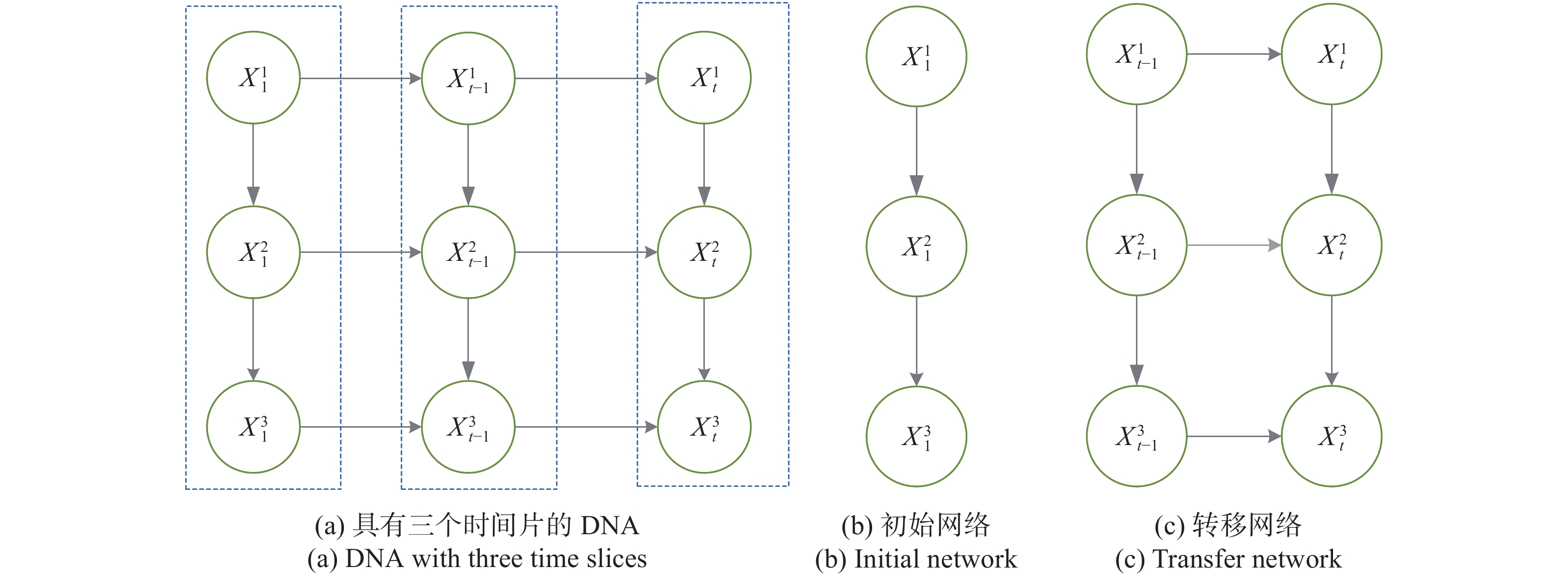
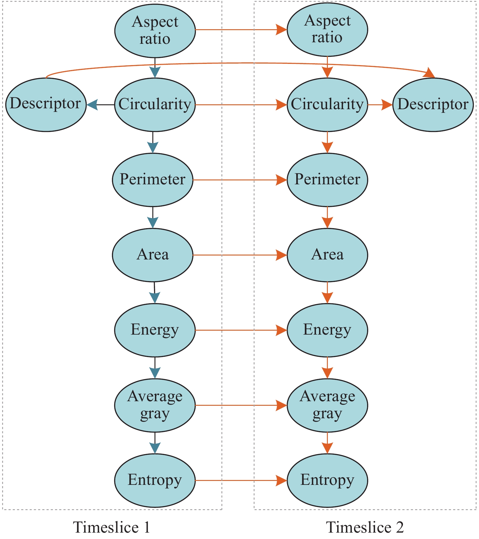
首先，定义特征$X_t^1,X_t^2,X_t^3, \cdots ,X_t^i$表示为第$ t $个时间片上的第$ i $个特征节点，如长宽比、周长、能量、面积、圆形度、灰度均值、熵等特征。

其次，如图1 (a)所示，定义时空关联推理网络（$ {B_1},{B_ \to } $），表示特征变量在时空约束先验条件下的特征关联。其中$ {B_1} $是初始网络，表示同一时刻不同特征间的依存关系，如图1 (b)所示，定义了初始时刻的概率分布。$ {B_ \to } $是转移网络，仅表示不同时刻下相同特征间的关联，如图1 (c)所示，定义了两个相邻时间片各变量之间的条件分布。两个相邻时间片间满足一阶马尔科夫假设，片内特征变量除了在t时刻被其他特征影响之外，还会受到相同特征在t−1时刻的影响，即：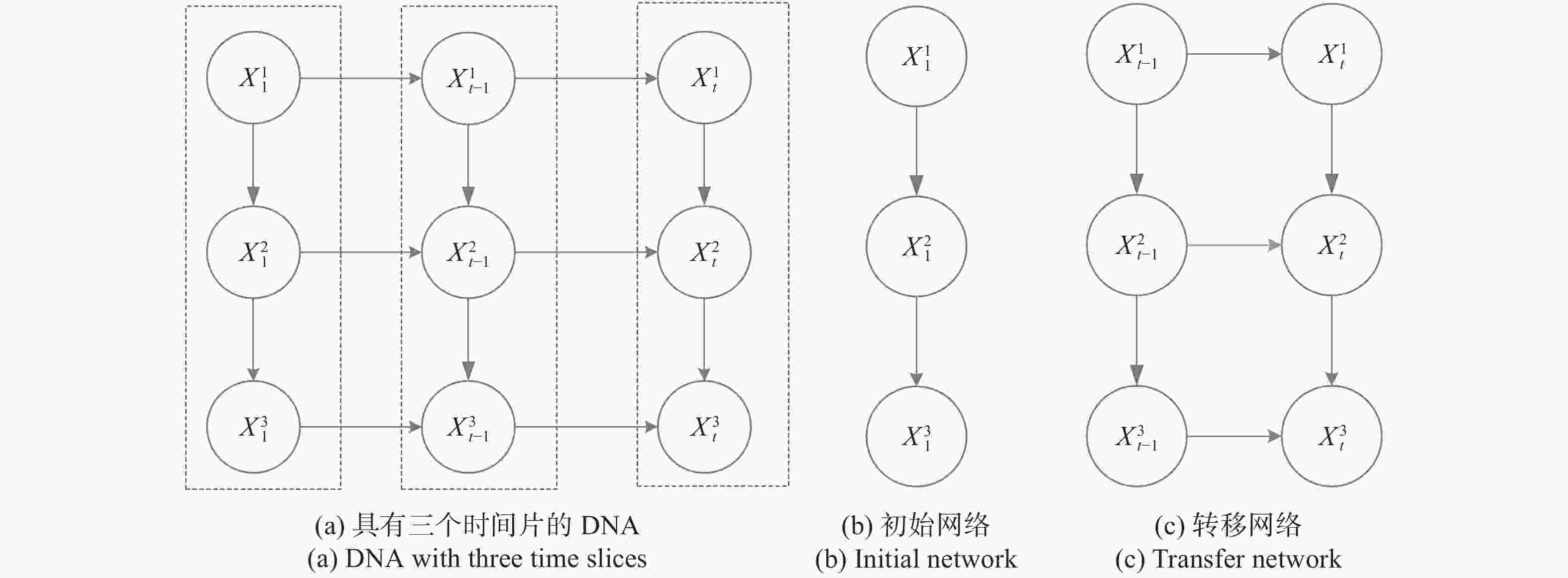

Figure 1.  Representation diagram of space-time correlation inference network

式中： $P{{a}}\left(X_t^i\right)$ 为特征 $ X_t^i $ 的父节点；$ {B_ \to } $ 中第二个时间片中的每个节点都有一个条件概率分布 $P\left(X_t^i|P{{a}}\left(X_t^i\right)\right)$，t>0 。特征节点 $ X_t^i $的父节点 $P{{a}}\left(X_t^i\right)$可以和 $ X_t^i $ 在同一个时间片内，也可以在前一个时间片内。位于同一个时间片内可以理解为特征变量之间相互影响，而跨越时间片的可以理解为特征变量随时间的变化规律。

最后，根据下述公式计算当前所预测目标与所有分类的匹配程度，匹配值最高的即为预测目标所属类别：

式中：$P\left(X_{1:T}^{1:m}|C\right)$表示测试数据与类别$ C $匹配的程度；$ P(C) $为类别$ C $的先验概率。

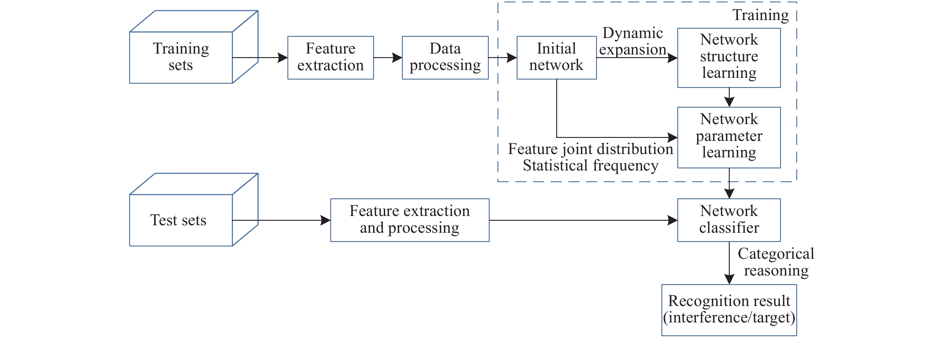
文中基于时空关联推理网络的抗干扰识别算法框架如图2所示。首先，构造训练样本数据集和测试集；其次，对训练样本的目标和干扰连通区域进行特征提取，构成的特征矢量记为：${A_i} = \left\{ {{X_1},{X_2},{X_3}, \cdots ,{X_1}_7} \right\}$；然后，将得到初始网络在两个连续的时间片上展开，针对当前时刻的特征变量引入上一时刻的该特征作为其父节点，计算相邻时间片各变量之间条件分布，由此得到转移网络，建立完整的时空关联推理网络结构；最后，将特征矢量输入时空关联推理网络分类器，得到对应连通区域的识别结果。

Figure 2.  Framework diagram of anti-interference recognition algorithm based on space-time correlation inference network

为进行样本空间构建，首先进行战场态势想定，弹道中目标高度固定为6 km，目标速度固定为0.8 Ma，导弹发射距离设定为7 km，干扰弹投射距离将2000~7000 m以500 m为间隔平均划分为11种情况，水平进入角将−180°~180°以5°为间隔平均划分为73种角度，投射策略按需要划分为九种，具体如表1所示。

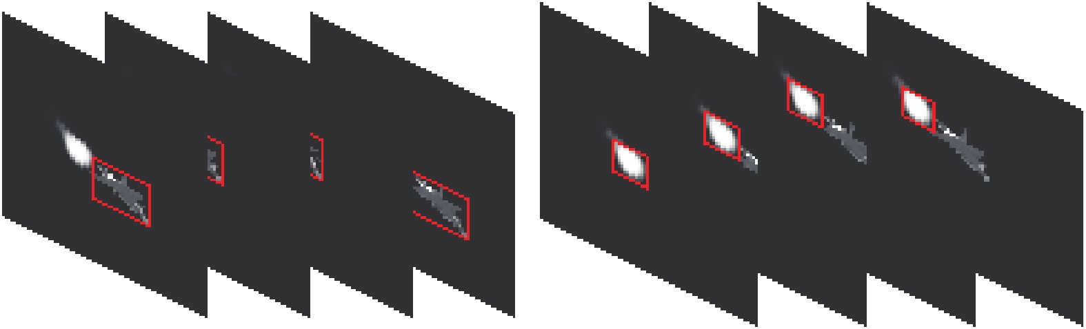
根据以上态势想定，共仿真7206条弹道，将弹道全过程输出格式为256×256的单通道16位灰度图序列。提取导引头图像序列，分别进行目标和干扰区域标注，以此作为正、负样本构造如图3所示的数据集。

Figure 3.  Schematic diagram of target and interference sample labeling

网络的节点对应一个随机变量，节点的取值既可以是连续的，也可以是离散的；有向弧代表了节点间的相互关系，两个变量之间存在依赖关系则用有向弧进行连接；节点的条件概率表用条件概率描述节点同其父节点的依赖关系的强弱。在文中，一个时间片包含17个特征节点，每个节点对应一个特征变量，其中包括长宽比、周长、能量、面积、圆形度、灰度均值、熵、傅里叶描述子分量1~10等特征。根据特征节点以及特征之间的关系、条件概率表，初始网络可以得到所有特征节点的联合概率分布。

基于构造的数据集，分别进行正、负样本图像特征提取，每一个样本${A_i}$对应一组特征矢量${A_i} = \left\{ {{X_1},{X_2},{X_3}, \cdots ,{X_{17}}} \right\}$，形成以特征矢量为形式的正、负样本库${S_ + } = \left\{ {{A_1},{A_2},{A_3}, \cdots ,{A_P}} \right\}$和${S_ - } = \left\{ {{A_1},{A_2},{A_3}, \cdots ,{A_Q}} \right\}$。基于该样本库构建初始网络分类器的网络。

首先，计算任意特征对之间的条件互信息，对所选取的17个特征节点两两进行条件互信息计算。条件互信息计算公式如下：

式中：${x_i}$、$c$分别表示特征节点${X_i}$和类别节点$C$的取值

其次，以所有特征节点为顶点构建完全无向图，并将条件互信息标记为特征节点之间弧的权重，依据条件互信息值，从大到小对两两特征之间弧排序。

最后，在选择的弧不能构成回路的约束下进行弧的筛选，选择任意一个特征节点作为起点，将弧转换为有向边，构成有向无环图。

文中17个特征构成的初始网络如图4所示。

Figure 4.  Initial network structure diagram

一个动态贝叶斯网络^[21]通常由初始网络和转移网络构成，将初始网络在两个连续的时间片上展开，针对当前时刻的特征变量引入上一时刻的该特征作为其父节点，计算相邻时间片各变量之间条件分布，由此得到转移网络。文中采用的时空关联推理网络结构如图5所示。

Figure 5.  Network structure diagram based on space-time correlation inference

在时空关联推理网络中，特征变量有两种条件依赖性。第一种，每个时刻的 $ {X_i} $ 特征节点指向当前时刻 $ {X_j} $ 节点的有向弧表示当前时刻不同特征节点之间的关系；第二种，连接 $ t - 1 $ 时刻的 $ {X_i} $ 特征节点和 $ t $ 时刻 $ {X_i} $ 节点的有向弧表示一个单独的特征节点随时间的发展情况。

因此，构建的时空关联推理网络能够充分运用目标和干扰识别过程中的特征时变规律，利用特征变量之间的概率关系模拟特征的动态发展，并且形成一个符合特征时空约束下的推理演化模型。

前文的结构学习获得了特定域中每一特征变量间的相互约束关系，在此基础上需要完成参数学习过程。参数学习^[22]是在给定网络结构的前提下获得相关变量之间的条件概率分布函数，表现为给定其父节点状态时该点取不同值的条件概率表，定量刻画了特征之间的依赖强度。

如果假设任意特征变量 ${X_i}(0 \leqslant i \leqslant N)$ 有 ${r_i}$ 种取值情况，其父节点 $Pa({X_i})$ 变量有 ${q_i}$ 种取值情况，则该特征变量的参数向量为 $\theta = \{ {{\theta _{ijk}}| {i = 1,\cdots,N; j = 1,\cdots,{r_i};}} {{k = 1,\cdots,{q_i}}} \}$，注意$\sum\nolimits_j {{\theta _{ijk}}} = 1\forall i,k$，表示任意特征变量取值的概率和为1。将满足 $p\left( {{X_i}\left| {Pa({X_i}) = k} \right.} \right)$ 的参数向量表示为 ${\theta _{i,k}} = \left\{ {{\theta _{ijk}}\left| {j = 1,\cdots,{r_i}} \right.} \right\}$。则要估计的参数为：

参数学习主要通过样本数据统计来实现，该算法采用最大似然估计法。根据对数似然估计法可以得到：

式中：$ {N_{ijk}} $代表满足$ {\theta _{ijk}} $的样本数量。

在参数学习过程中，将时空关联推理网络看成是扩展的由时间变量联系在一起的两片初始网络组成，除了对每一片利用样本数据估计特征节点条件概率表，表2所示为其中面积特征节点的片内条件概率表，也需要估计特征节点两片之间的转移概率，表3所示为其中面积特征节点的转移概率表。

时空关联推理网络满足齐次性假设，即$ {B_ \to } $中的参数不随时间而发生变化，根据初始分布和相邻时间片之间的条件分布，可以将时空关联推理网络展开到第T个时间片。

由于离散时空关联推理网络符合条件独立性假设，可得到时空关联推理网络初始时刻的概率分布为：

式中：将$\left\{ {X_{t - 1}^1,X_{t - 1}^2, \cdots X_{{{t - 1}}}^m} \right\}$记为$X_{{{t - 1}}}^{1:m}$；$pa(X_{t - 1}^i)$表示$X_{t - 1}^i$的父节点集合。

两个相邻时间片各变量之间的条件分布为：

式中：$ X_t^i $ 为第$ t $个时间片上的第$ i $个节点；$ Pa(X_t^i) $为 $ X_t^i $ 的父节点。第二个时间片中的每一个节点都有一个条件概率分布 $P\left(X_t^{\text{i}}|Pa\left(X_t^i\right)\right)$， t>0。节点$ X_t^i $的父节点 $ Pa(X_t^i) $ 可以和 $ X_t^i $ 在同一个时间片内，也可以在前一个时间片内。

根据时空关联推理网络的齐次性假设，得到一个跨越多个时间片的联合概率分布：

式中：$ T $为时空关联推理网络包含时间片个数；$ m $为一个时间片包含的节点数。

时空关联推理网络的贝叶斯公式为：

式中：$P\left(X_{1:T}^{1:m}|C\right)$ 表示测试数据与类别 $ C $ 匹配的程度；$ P(C) $ 为类别 $ C $ 的先验概率。

对于一组特征值$A_{1:2}^{1:17} = \left\{ X_1^1,X_1^2,X_1^3,\cdots ,X_2^{17}\right\}$，依据上节得到的每一个属性节点的片内条件概率表以及片间转移概率表，分别计算$ P(A_{1:2}^{1:17}|{C_i}) $，$ i = 1,2 $及每个类的先验概率$ P({C_i}) $。

通过比较$ P(A_{1:2}^{1:17}|C = 0) \cdot P(C = 0) $和$P\left(A_{1:2}^{1:17}|C = 1\right) \cdot P\left(C = 1\right)$得到对于样本$A_{1:2}^{1:17} = \{ X_1^1,X_1^2,X_1^3,...,X_2^{17}\} $的时空关联推理网络检测结果。若$P\left(A_{1:2}^{1:17}|C = 1\right) \cdot P(C = 1) > P\left(A_{1:2}^{1:17}|C = 0\right) \cdot P\left(C = 0\right)$，则该样本属于目标，反之则属于干扰。

综上所述，文中算法首先标记连通区域分割疑似目标区域，提取区域时空特征信息并采用动态贝叶斯推理网络识别目标，实现目标抗干扰识别。

网络训练步骤如下：

Input：training data set M

for i ← sizeof (M)

m_i ←feature extraction (m_i)　　m_i ← data processing(m_i)build dynamic Bayesian networks　　table of probability ← train DBN(M)　　End

Output：table of conditional probability

推理识别步骤如下：

Input：test data set X

for i ← sizeof (X)

x_i ← image preprocessing(x_i)　　r(j) ←labeling connected regions(x_i)　　for j 　　　A_j ← feature extraction(r_j) 　　　P (Target, Interference) ← Table (A_j)　　　if P (Target) > P(Interference) then　　　　　A_j is target 　　　else　　　　　A_j is interference　　　if (x_i contain Target and Target is right) then 　　　　 N_right=N_right +1 　　else 　　 　　 N_false=N_false +1 　　　 P (right) ← caculate (N_right, N_false) 　　 End

Output：Recognition rate P(right)

仿真测试数据集包括初始发射条件、目标机动、干扰投射策略三个维度的对抗条件参数，该实验所用图像数据集的对抗条件参数的量化共包含12个：

（1） 对抗态势有七个参数：目标高度、载机高度、目标速度、载机速度、水平进入角、发射距离、综合离轴角（可分解为水平离轴角、垂直离轴角）；

（2） 目标机动有五种类型：无机动、左机动、右机动、跃升、俯冲；

（3） 红外干扰投放策略四个参数：总弹数、组数、弹间隔、组间隔。

因此，文中设置的仿真图像序列生成条件如下：

（1） 导弹发射距离为7000 m；

（2） 目标高度及载机高度均为6000 m；

（3） 红外点源干扰弹总数为24枚；

（4） 目标机动类型为无机动、左转、跃升；

（5） 组间隔为1.0 s，投弹组数分别为12、6；

（6） 水平进入角选取典型的±10°、±40°、±70°、±100°、±130°、±160°。

基于以上参数设置，使用红外仿真平台产生逼近实际空战对抗环境的仿真图像，数据的输出格式为256×256的单通道16位灰度图序列。

定义识别率如下：

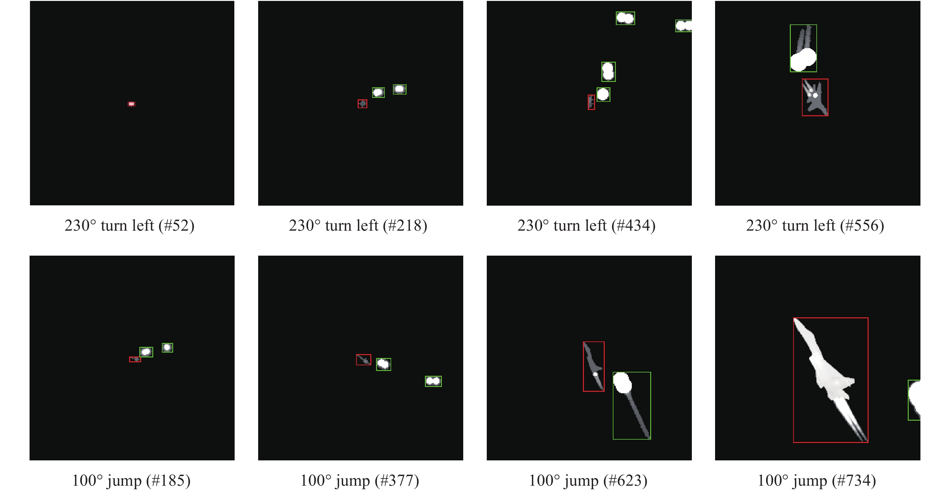
式中：${N_{right}}$表示正确识别的目标数；${N_{total}}$、${N_{false}}$分别表示总目标数和干扰被错判为目标的数量。

用时空关联推理网络分类器对多种态势下的飞机和干扰进行识别，部分结果如图6所示，结果中，将飞机用红色矩形框标出，干扰用绿色矩形框标出。利用识别率公式计算图像序列的识别率以定量描述算法的识别性能，如表4所示。

Figure 6.  Test chart of target recognition algorithm based on space-time correlation inference network

在该次实验中一共选取了25465张测试图片，采用基于时空关联推理网络的识别算法，最终统计结果为识别目标数为23937，虚警数为617，目标识别率为94%。

测试结果表明，在以上测试条件下，时空关联推理网络具备点源人工诱饵全程对抗能力，导弹的识别率达到94%。

文中基于时空关联推理网络结构研究了空战环境下的目标识别问题。在已测试的空战干扰对抗仿真图像数据集下，仿真实验结果表明基于时空关联推理网络算法识别率达到94%，比基于TAN分类器的抗干扰识别算法高3%。基于时空关联推理网络的抗干扰目标识别算法能够在一定程度上解决假目标、目标遮挡等难题，对全程抗干扰也有一定的效果，但效果并不理想。下一步工作，一方面需要扩充样本库，补充目标与干扰粘连的样本，得到更为准确的先验信息；另一方面需要解决目标与干扰粘连时如何对目标与干扰特征进行区分，进行更多特征之间关系的挖掘，特别是外形轮廓特征及具有不变性质的特征，使得对目标和干扰的描述更加全面与稳定。