Pose estimation of camera based on weighted accelerated orthogonal iterative algorithm

相机位姿估计在计算机视觉、机器人、摄影测量中有广泛的应用^[1]，常用的方法是在相机内参已知的情况下，通过n个空间参考点与其所对应的图像点来估算相机的空间位置和姿态信息，这通常称为n点透视问题，即PnP (perspective-n-point)问题^[2]。

目前，求解PnP问题的算法主要分为非迭代算法和迭代算法^[3]。非迭代算法计算速度快，但对噪声敏感，一般得不到较高的位姿精度。其中具有代表性的算法有DLT （direct liner transformation）算法^[4]、EPNP （efficiency PnP）算法^[5]、RPnP （robust PnP）算法^[6]、OPnP （non-iterative PnP）算法^[7]、SRPnP （single gaussian-newton robust PnP）算法^[8]等。迭代算法通过迭代计算位姿，精度较高，但也因此耗时较久，并且初始位姿的选取对最终的结果影响较大，容易收敛到局部最优值。迭代算法的代表有比例正交投影迭代变化（pose from orthography and scaling with iterations，POSIT）算法^[9]，以及正交迭代（orthography iterative，OI）算法^[10]。由于采用了奇异值分解(Singular Value Decomposition，SVD)，OI算法可以得到正交的旋转矩阵，并且OI算法引入了空间共线性误差的概念，相较于POSIT算法收敛性更好，在初始值不精确的时候也能保证收敛到不错的位姿，因此正交迭代算法成为目前应用较为广泛的位姿估计方法。

OI算法于2000年由Lu等^[10]提出的，后续经过了不断的发展完善。2009年，Zhang等^[11]提出了基于直线的正交迭代算法（LBOI），将OI算法中的点与点的对应推广到了直线形式；Didier等^[12]提出了基于正交迭代算法的混合姿态估计方法（COI），通过正方形基准定位技术获取姿态初值带入到正交迭代算法中从而加快算法收敛速度并提高精度。2015年，李鑫等^[13]提出了一种加速正交迭代算法（OI+），通过规整正交迭代算法中计算过程，加速正交迭代算法从而减少算法运行时间。2017年，Huo等^[14]提出了基于不确定加权测量误差的特征目标位姿估计的广义正交迭代算法（GOI），将正交迭代算法推广到立体视觉系统中进行位姿估计。2018年，Sun等^[15]提出了基于入射射线跟踪模型的正交迭代算法(PROI)，用入射射线跟踪摄像机模型替代原有的针孔相机模型；周润等^[16]提出了加权形式的正交迭代算法。2019年，Dong等^[17]提出了soft+OI的组合算法，将SoftAssign算法与OI算法结合，可以在不确定物点与像点的对应关系的情况下，同时得到位姿和物点与像点的对应关系；张雄峰等^[18]提出了基于S估计的加权正交迭代算法，通过S估计法计算权值从而加强算法的鲁棒性。OI算法经过推广扩大了其使用范围，但由于迭代过程复杂，耗时较多，实际应用中受到一定制约。

为了提高OI算法的求解精度并且降低计算时间，提出了一种加权加速正交迭代算法（WAOI），关键思想在于构建加权形式的目标函数，通过物方重投影误差调整权重系数，优化位姿估计结果提升解算精度；通过自适应权值以及对迭代过程中冗余计算的整合，减少迭代过程中的计算量，实现算法的加速。

经典正交迭代算法的基本原理是物点、像点、相机坐标系原点三点共线^[10]，即满足共线性方程：

式中：P_i为第i个($i = 1, \cdots ,n,n \geqslant 4$)非共线参考点在目标坐标系下的三维坐标；${{\boldsymbol{V}}_{\boldsymbol{i}}} = \dfrac{{{v_i}v_i^t}}{{v_i^t{v_i}}}$为视线投影矩阵，v_i为第i个参考点在归一化像平面上的投影坐标；R为旋转矩阵；t为平移向量。以空间共线性误差平方和作为目标函数，通过最小化目标函数得到最优估计的R和t，目标函数定义为：

式中：I为单位矩阵。经典正交迭代算法中赋予每个参考点的权值是相同的，因此当测量数据中存在粗大误差时，会对最终的姿态估计精度产生较大影响。为了提高正交迭代算法的精度，考虑加权形式的正交迭代算法，通过对误差较大的参考点赋予较小的权值，来减小误差较大的点对最终位姿估计精度的影响^[16]。加权形式的目标函数为：

式中：第i个参考点的权值为${\omega _i}$。假设R的初始值为R⁽⁰⁾，第k次迭代时的R值为R^(k)，第i个参考点的权值为$\omega _i^{\left( k \right)}$。由公式（3）可知，目标函数为t的二次函数，因此在R^(k)和$\omega _i^{\left( k \right)}$的值确定后，可以得到第k次迭代的t^(k)的线性最优解为：

由R^(k)和t^(k)则可计算得到对应参考点的视线投影向量${\boldsymbol{q}}_{\boldsymbol{i}}^{\left( {{k}} \right)}$：

通过求解公式（6）的绝对定向问题得到R^(k+1))。R^(k+1)的具体解算步骤如下：定义${\boldsymbol{\overline P}} = \displaystyle\sum\limits_{i = 1}^n {\omega _i^{\left( k \right)}{{\boldsymbol{P}}_{\boldsymbol{i}}}} $，${\boldsymbol{\overline q}} = \displaystyle\sum\limits_{i = 1}^n {\omega _i^{\left( k \right)}{\boldsymbol{q}}_{\boldsymbol{i}}^{\left( {{k}} \right)}}$，则有：

参照经典正交迭代算法，定义$\boldsymbol{M}=\sum_{i=1}^{n} \omega_{i}^{(k)} \boldsymbol{q}_{i}^{k^{\prime}} \boldsymbol{P}_{i}^{\prime t}$，对M进行SVD分解，则有：

当${{\boldsymbol{R}}^{\left( {{{k + 1}}} \right)}} = {\boldsymbol{U}}{{\boldsymbol{V}}^{{{\rm{T}}}}}$时，公式（6）取得最小值，此时物方残差和最小，因此可以得到R^(k+1)。重复上述计算过程，直至R和t满足收敛条件，从而得到R和t的最优估计。

参考点的权值，采用物方重投影误差来确定。即通过计算参考点在相机位姿估计结果下的物方投影误差，利用收敛速度快的改进Huber函数^[19]确定权重系数；对投影误差大的参考点，认为其测量误差较大，对其分配较小权重，以提高位姿估计精度。具体步骤如下：各参考点初始权值均设为1/n，设第k次迭代时第i个参考点的权值为$\omega _i^{\left( k \right)}$，利用1.1节的方法计算得到旋转矩阵R^(k)和平移向量t^(k)，由公式(5)、(7)、(8)得到各参考点的物方投影误差：

利用改进型Huber函数更新各参考点权值系数，改进型Huber函数的表达式为：

式中：$r = \dfrac{1}{n}\displaystyle\sum\limits_{i = 1}^n {r_i^{\left( k \right)}} $。重复上述迭代过程，直到权重系数满足收敛条件为止。

加权正交迭代算法由于每次迭代需要计算各参考点的物方投影误差并更新权值，因此计算耗时较经典正交迭代算法较长。由仿真实验可知，一般权值的调整在迭代一定次数便趋于稳定，因此考虑在权值收敛后将权值设为定值，从而减少算法迭代过程中的计算量；进一步的，通过整合固定权值的加权正交迭代算法中的冗余计算，加快计算效率实现算法加速。具体加速步骤如下：

（1）自适应权值。计算两次迭代的参考点权值之差的模，若小于设定阈值则认为权值已收敛，此时将权值设为最后一次更新的值，后续计算将不对权值进行更新，以减少计算量。

（2）整合迭代过程中的冗余计算。当参考点权值为定值后，由公式(4)可知，t可由R线性解出，投影点和目标函数均为R和t的函数，因此可以用R表示。通过对迭代过程中计算的规整化，将重复计算的部分用常系数矩阵表示，在迭代过程前计算，减少迭代过程中的计算量进而加快迭代过程。

为了计算方便，引入矩阵计算公式：

式中：$vec\left( {} \right)$表示将矩阵按照列堆栈形成的向量；$ \otimes $表示Kronecker积。

首先对参考点进行零均值化，${{\boldsymbol{P}}_{{i}}}' = {{\boldsymbol{P}}_{{i}}} - \overline {\boldsymbol{P}}$，$\overline {\boldsymbol{P}} = \displaystyle\sum\limits_{i = 1}^n {{{\boldsymbol{\omega }}_{{i}}}{{\boldsymbol{P}}_{{i}}}}$，根据最优t的计算以及公式(12)，则有：

其中，${{\boldsymbol{r}}^{\left( {{k}} \right)}} = vec\left( {{{\boldsymbol{R}}^{\left( {{k}} \right)}}} \right)$

则计算后的投影点坐标为：

在利用绝对定向问题求解最优姿态时需要计算矩阵M。

式中：$\overline {{{\boldsymbol{q}}^{\boldsymbol{k}}}} $为第k次迭代时所有投影点的平均值，令${{\boldsymbol{m}}^{\left( {{k}} \right)}} = vec\left( {{{\boldsymbol{M}}^{\left( {{k}} \right)}}} \right)$，则有：

其中

根据绝对定向最优解，对其进行奇异值分解${{\boldsymbol{M}}^{\left( {{k}} \right)}} = {\boldsymbol{U\Sigma }}{{\boldsymbol{V}}^{\rm{T}}}$，则得到R的最优估计${{\boldsymbol{R}}^{\left( {{{k + 1}}} \right)}} = {\boldsymbol{U}}{{\boldsymbol{V}}^{\rm{T}}}$，然后继续进行下一次迭代。

针对目标函数的优化，则有：

其中

参考点P_i均为零均值化后的参考点，经过上述计算整合后，每次迭代时可由矩阵F计算得到M，再利用奇异值分解得到最优旋转矩阵R。目标函数的计算可以通过G确定，当权值为定值时，F、G为常系数矩阵，因此可以在迭代过程之前进行计算，从而减少计算量，达到加速的目的。

对于迭代算法而言，必须给出收敛性证明。根据全局收敛定理^[20]，算法收敛需要满足3个条件。

（1） WAOI计算结果是封闭的。

（2） WAOI每次迭代产生的R都是封闭的。

（3） WAOI误差函数在迭代中严格单调下降，直至达到最终收敛条件。

对于第一个条件，正交迭代算法可分为3个映射，计算M矩阵，M矩阵的SVD分解，R的计算，可以看出上述3个步骤的计算都是连续且封闭的，封闭映射的组合依然是封闭的，因此WAOI也是封闭的。

WAOI每次迭代计算出的R都是正交矩阵，封闭且有界，因此第2个条件也是满足的。

对于WAOI误差函数严格单调性的证明，首先给出误差函数的表达式：

通过R^(k)的计算公式(9)，可知R为使得公式(9)取最小值时的值，因此有：

由公式(21)、 (22)可得：

假设R^(k)不是WAOI算法的收敛点，则有${{\boldsymbol{R}}^{\left( {{{k + 1}}} \right)}} \ne {{\boldsymbol{R}}^{\left( {{k}} \right)}}$，${\boldsymbol{q}}_{{i}}^{\left( {{{k + 1}}} \right)} \ne {\boldsymbol{q}}_{{i}}^{\left( {{k}} \right)}$，进而可以得到$\displaystyle\sum\limits_{i = 1}^n {{{\left\| {{{\boldsymbol{V}}_{{i}}}{\boldsymbol{q}}_{{i}}^{\left( {{{k + 1}}} \right)} - {{\boldsymbol{V}}_{{i}}}{\boldsymbol{q}}_{{i}}^{\left( {{k}} \right)}} \right\|}^2}} \ne 0$，$E\left( {{{\boldsymbol{R}}^{\left( {{{k + 1}}} \right)}}} \right) \lt E\left( {{{\boldsymbol{R}}^{\left( {{k}} \right)}}} \right)$，从而得到WAOI误差函数是严格单调下降的，因此可以证明WAOI是严格收敛的。即从任意数值的初始值，WAOI都能收敛到一个固定值。

仿真实验中相机内参参照真实相机设置，等效焦距为2500，图像分辨率为2590 pixel×2 048 pixel。参考点在相机坐标系下的坐标等间距分布在[−10 cm，10 cm]×[−10 cm，10 cm]×[300 cm，310 cm]的区域内。平移向量选择为参考点的中心。旋转矩阵的迭代初始值R⁽⁰⁾，一般通过弱透视投影模型计算得出，为了进一步增加WAOI算法的全局收敛性，且加快收敛速度，选取目前非迭代算法中精度较高且运行速度较快，具有全局寻优的SRPnP算法，将其位姿解算值作为旋转矩阵迭代初始值R⁽⁰⁾。对参考点对应的像点添加均值为0，标准差为0.1 pixel的高斯噪声模拟图像处理误差。仿真平台为Matlab R2017 a；CPU型号为Intel(R)Core(TM) i5-9400 F，主频2.90 GHz；内存16 GB。为便于评定位姿解算精度，定义旋转矩阵误差e_R与平移向量e_t误差如下：

式中：R和R_true分别表示旋转矩阵解算值和真实值；t和t_true分别表示平移向量解算值和真实值^[3]。对每种情况，进行姿态解算独立重复试验1000次。

为比较不同算法之间的性能，将文中的WAOI与提供迭代初值的SRPnP ^[8]、经典正交迭代算法OI ^[10]、加权正交迭代算法WOI ^[16]分别进行比较，从参考点数目、噪声水平、粗差点数目以及运行时间4个方面进行对比。

(1）参考点数目

取参考点数目范围4~25，在参考点中随机选取两个点，对其图像坐标添加标准差为1 pixel的高斯噪声模拟粗差，分别用上述4种算法进行姿态解算，旋转矩阵与平移向量解算结果如图1所示。

Figure 1.  Curve of attitude calculation error with the number of reference points

由图1（a）可以看出，随着参考点数的增加，四种算法的旋转矩阵误差均在减小，在参考点数目大于4时，文中提出的WAOI在旋转矩阵的解算精度上高于SRPnP和OI，与WOI近似；由图1（b）可以看出，在平移向量的解算精度上，WAOI的解算精度高于其他所有算法，这是因为WAOI采用了物方投影误差作为权重系数的确定依据，与WOI的像平面投影误差相比，在平移向量的解算上会有较好的精度。WAOI仅在参考点数目为4时姿态解算精度不及SRPnP和OI，这是因为WAOI通过给粗差点赋予较小的权值以减弱其对最终解算精度的影响，这在参考点数目比较少的时候会造成参与计算的参考点数目不足从而造成比较大的解算误差。

（2）噪声水平

将参考点数目固定为25个，粗差点数固定为两个，改变粗差点噪声水平，得到姿态解算误差随噪声变化曲线如图2所示。由图2（a）可以看出，在旋转矩阵解算上WAOI和WOI均对噪声有较强的鲁棒性，旋转矩阵解算误差基本不随噪声水平变化，与SRPnP和OI对比具有较大的优势；图2（b）中平移向量解算误差与图2（a）中旋转矩阵误差类似，WAOI和WOI的平移向量解算误差基本不随噪声水平变化，并且WAOI相较于WOI精度略高。

Figure 2.  Attitude calculation error varying with noise level

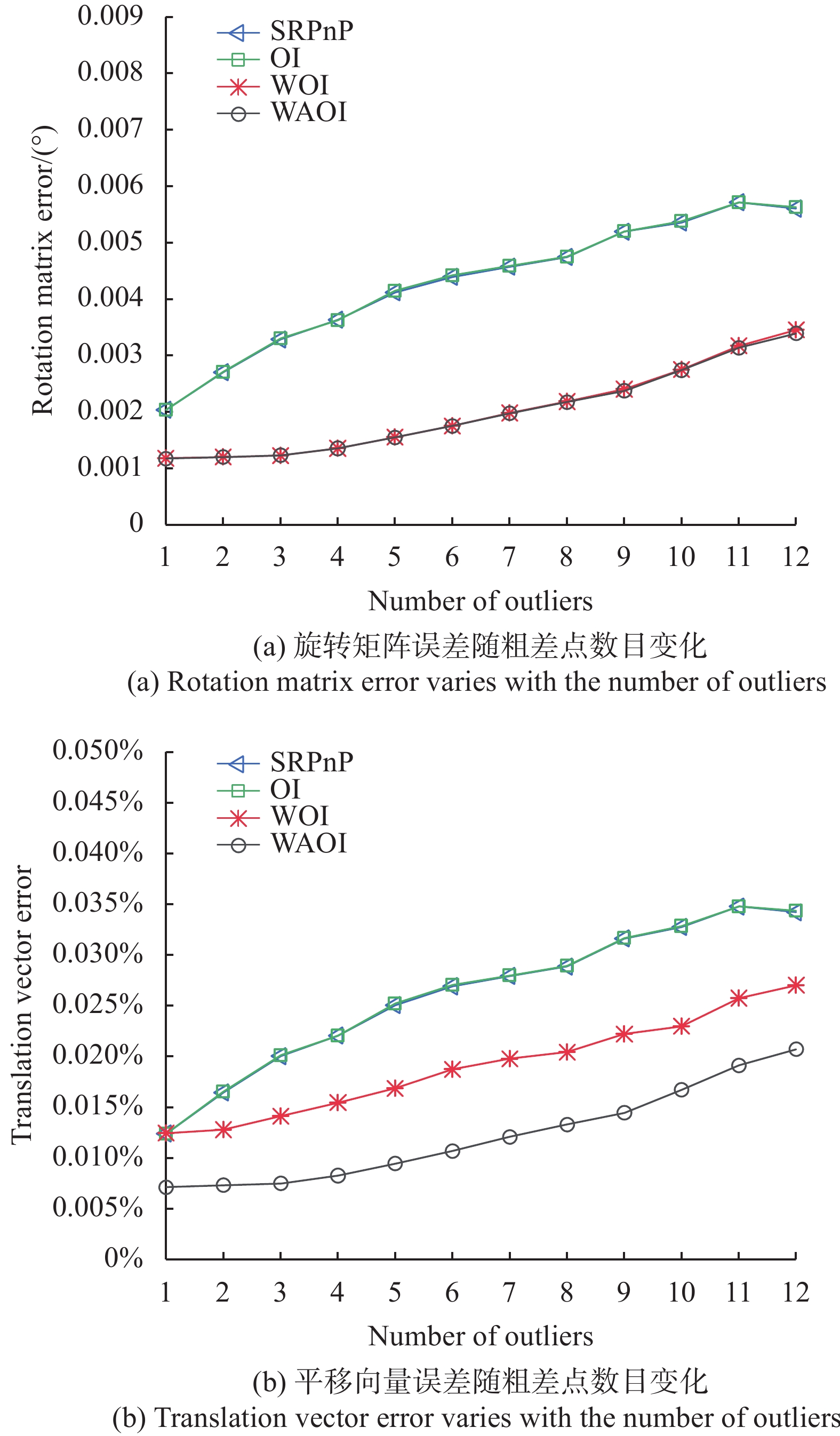
(3）粗差点数目

固定粗差点的高斯噪声水平不变，改变粗差点的数量，得到姿态解算误差随粗差点数目变化曲线如图3所示。由图3（a）可以看出，随着噪点数目的增多，4种算法的旋转矩阵误差均有所增大，WAOI与WOI算法精度相近，旋转矩阵误差约为OI和SRPnP的一半。由图3（b）可以看出，4种算法的平移向量误差也会随粗差点数量增多而加大，解算精度方面，WAOI优于其余3种算法。

Figure 3.  Attitude calculation error changing with the number of outliers

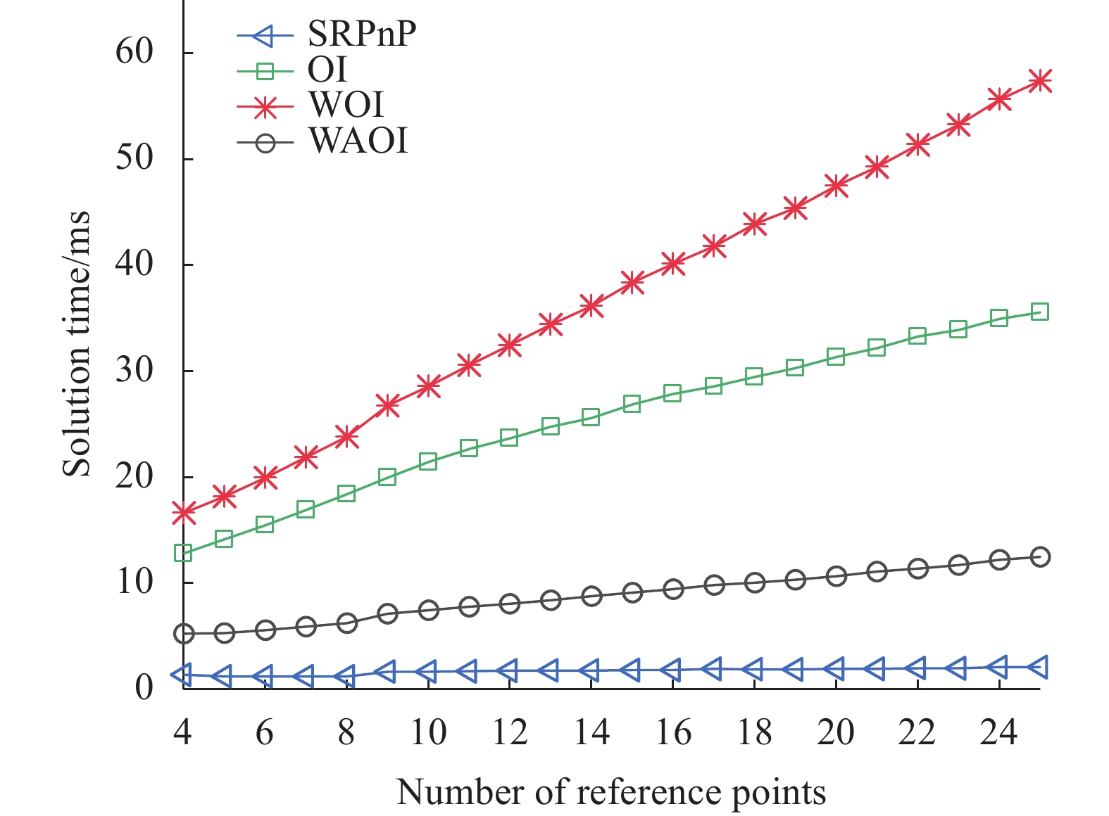
(4）运行时间

4种算法的解算时间随参考点数目变化如图4所示，由此可以看出，非迭代的SRPnP的计算时间最少，且对参考点数目不敏感。迭代算法中WAOI耗时最少，其次是OI，耗时最长是WOI。

Figure 4.  Solution time varies with the number of reference points

文中的WAOI优化了计算过程，通过自适应权值，整合迭代中的计算过程，显著降低了计算耗时。在参考点数目为4个时，WAOI相较于OI耗时较低了59.11%，相较于WOI耗时降低了68.52%；在参考点数目为25个时，WAOI相较于OI耗时较低了64.83%，相较于WOI耗时降低了78.21%。随着参考点数目的增多，WAOI的解算效率的优势越发明显。

仿真实验表明，当测量数据中存在粗差时，WAOI与SRPnP和OI相比，旋转矩阵以及平移向量均能达到较高的精度；与WOI相比，旋转矩阵精度相近，平移向量精度略高，表明WAOI在算法鲁棒性方面具有良好的效果，在数据存在噪声的情况下依然能获得较高的解算精度。在算法耗时方面，WAOI相较于OI和WOI均实现了较大的超越，速度较快，实时性较好。

实验中相机选用德国Balser ace acA2500-20 gm，分辨率为2590 pixel×2 048 pixel，水平像元尺寸与垂直像元尺寸均为4.8 μm，镜头焦距为12 mm，相机的内参以及畸变参数由相机标定得到^[21]。使用12个固定参考点，通过相机拍摄参考点图像，实验装置如图5所示，计算机配置与仿真实验相同。

Figure 5.  Experiment equipment

随机选取两个参考点添加噪声模拟粗差。通过4种算法解算得到位姿参数，计算参考点的像平面重投影结果，通过比较重投影结果与实测值来反映位姿解算精度^[22]。由于WOI与WAOI精度相近，重投影图中不易分辨，因此不包含WOI。参考点在像平面上的重投影结果如图6所示。

Figure 6.  Reprojection results of image plane

从图6可以看出，WAOI对应的解算结果与测量结果非常接近，而SRPnP和OI的解算结果与测量结果有较大的偏差。进一步分析各方法测量精度差异，计算12个参考点重投影位置如表1所示，其中x、y分别为参考点在像平面像素坐标，r为参考点重投影结果与测量结果之间的距离。

从表1可以看出，WAOI解算得到的参考点重投影均方根误差为0.64 pixel，SRPnP和OI分别为10.29 pixel和11.18 pixel。WAOI与SRPnP和OI相比，参考点重投影结果与测量结果之间的距离要低一个数量级，表明WAOI的位姿解算精度更高。此外解算时间方面，OI平均耗时为23.64 ms，WOI平均耗时为31.89 ms，WAOI平均耗时为8.02 ms，实验表明，WAOI与OI和WOI相比，运算效率分别提升了66.07%和74.85%，具有明显优势。

文中提出了一种用于相对位姿标定的加权加速正交迭代算法，利用加权共线误差作为目标函数，通过物方投影误差更新权值，利用自适应权值和整合迭代过程加快收敛过程，优化位姿估计结果，具有精度高，鲁棒性好，实时性好的优点。仿真分析和实验结果表明，WAOI的姿态解算精度随噪声影响较小，在强噪声水平下依然可以达到较高的精度，鲁棒性好，相较于WOI提升了平移向量解算精度。在12个参考点中存在两个粗差点的情况下，WAOI的参考点重投影精度为0.64 pixel，与SRPnP和OI相比高一个量级；运算时间为8.02 ms，运算效率与OI相比提升了66.07%，与WOI相比，提升了74.85%，实时性好，具有较强的工程实用价值。