Light field camera modeling and distortion correction improvement method

传统相机的成像方式只能记录光线所经过的位置信息，丢失了光线的深度信息，即三维信息。光场相机作为一种新型成像系统，由于其内部含有微透镜阵列这一特殊构造^[1]，可以同时获取光线的角度和位置信息，能颠覆传统成像方式的图像生成方法，实现如数字重聚焦、合成子孔径图像、光场显微成像、全景深图像合成、场景深度图获取等功能^[2]。能够为三维重建^[3]、全景拼接、视角合成、目标识别与跟踪等计算机视觉问题提供更加完备而有效的解决方案^[4]。

光场相机的原型首先是由Adelson和Wang^[5]在1992年提出的。第一个商业化的手持光场相机是由Ng R^[6]在2005年设计的，然后由Lytro公司发布。该光场相机在图像传感器与主透镜之间放置了一个微透镜阵列，通过它来获取光线的更多场景信息。但是该相机模型的空间分辨率不高，又被称为未聚焦光场相机。2009年，Georgiev 和 Lumsdaine^[7-8]提出了基于Ng光场相机模型的新模型，名为聚焦光场相机，其中微透镜阵列（MLA）聚焦于主透镜形成的图像平面上。这个相机模型由Raytrix公司发布，有更高的空间分辨率，但是角度分辨率较低。

相机的标定参数可以提高其精度和性能，因此，研究者们提出了不同的标定方法。2013年，Dansereau^[9]等人提出一种包含15个参数的相机标定模型和方法，他们推导了像素索引与光线的四维内参矩阵和畸变模型，但其工作中仍然存在着初始化优化和解决校准参数等问题。2014年，Bok^[10]等人提出了利用原始图像提取适当区域内线的特征校正线性形状的相机投影模型的方法，然而，他们并没有模拟外子孔径图像的镜头畸变。2016年，Zeller^[11]等人提出了一种测量校准方法，使用全聚焦图像和虚拟深度图计算三维观测结果，然而，该方法未能得到物体距离超过1 m的特征点。Johannsen^[12] 等根据该特征重建标定物的三维点坐标，通过序列二次规划（SQP）优化方法求解内外参数，但却忽略了微透镜产生的畸变。Zhang^[13]等人提出了一种基于原始图像特征与深度尺度信息之间关系的校准方法，然而他们没有对微透镜阵列引起的畸变误差进行补偿，为了填补这一空白，2017年，Noury^[14]等人提出了一种仅基于原始图像的校准方法。这项工作开发了一种新的检测器，以直接估计棋盘格，观察原始图像的亚像素精度。然而，他们从白图像而不是捕获的原始图像估计微图像的网格参数，这在标定过程中引入了不确定性。光场相机出现时间不长，其成像模型的建立与参数标定研究并不多，仍然不成熟。

文中在经典的Dansereau方法的基础上，改进了光场相机的标定与畸变校正方法，通过通用的小孔成像与薄透镜模型，分析了光场相机模型中参数的物理意义，并用通用相机的标定方法进行光场相机标定，推导出不同方向的子孔径图像像素坐标的索引与穿过主透镜和微透镜阵列的光场射线的精确关系，利用投影转换关系估计出光场相机的内参，并考虑相机的径向畸变与切向畸变模型，最后利用重投影误差对其参数进行优化。

光场相机的典型代表是Ng等设计的传统光场相机（Plenopic 1.0）。小孔成像模型描述微透镜阵列，薄透镜模型描述主镜头。该成像装置在传统相机的焦平面处放置一个微透镜阵列，并将图像传感器置于微透镜的一倍焦距处。真实场景中特定深度平面上来自同一点的不同方向光束，通过主镜头折射、微透镜聚焦，最终被图像传感器上的成像单元所记录，如图1所示。

如图1所示，$ A $表示图像传感器平面，$ B $表示微透镜阵列平面，C表示主透镜平面，$O - XY$为图像坐标系，${O_c} - {X_c}{Y_c}{Z_c}$为相机坐标系，${O_w} - {X_w}{Y_w}{Z_w}$为世界坐标系。光场相机模型表示为光线的路径，以穿过微透镜阵列平面及图像传感器平面的射线作为此光线的开始，即$n = {\left[ {i{\text{ }}j{\text{ }}k{\text{ }}l} \right]^{\rm{T}}}$，$ i $和$ j $为每个微透镜对应像元的索引，$ k $和$ l $为微透镜的位置索引，完整的转换过程如公式(1)所示^[9]。如果每个微透镜对应的像元像素为${N_i} \times {N_j}$，那么$ i $和$ j $的范围为$0 \sim {N_{i,j}}$；若有${N_k} \times {N_l}$个微透镜，则$ k $，$ l $的范围为$0 \sim {N_{k,l}}$。

Figure 1.  Geometric model of light field camera

为了便于说明，将四维坐标简化为横向的二维坐标，再延伸至四维光场，即$n = {\left[ {\begin{array}{*{20}{c}} i&k&1 \end{array}} \right]^{\rm{T}}}$。$H_{rel}^{abs}$是将相对坐标转换为绝对坐标的矩阵，即把$ i $转换为${i_{abs}}$，如图2所示，$ i $是相对坐标，表示每个微透镜下宏像素的索引，把相对坐标加上其对应的微透镜索引$k$处的实际像素，即$kN$，并减去宏像素的中心${c_{pix}}$就得到了绝对坐标${i_{abs}}$，其表示在图像传感器平面上相对坐标对应的微透镜图像的实际索引，转换过程为公式（3），$N$是每个微透镜下的宏像素大小，${c_{pix}}$是每个微透镜下的宏像素的中心，$ {c}_{pix}=N/2 $。

Figure 2.  The relative coordinates are converted to absolute coordinates

下一步是把绝对坐标转换为光场射线表示，此处与普通相机的小孔成像模型类似，首先通过$H_{abs}^\varphi$将绝对坐标${i_{abs}}$与微透镜阵列的索引$k$分别减去图像传感器和微透镜阵列的中心位置偏移量，再除以对应的单位物理尺寸（mm）可得到其在图像传感器平面与微透镜阵列平面实际的物理尺寸(mm)，$1/{F_s}$和$1/{F_u}$分别表示图像传感器像素和微透镜的单位物理尺寸(mm)，${c_m}$和${c_u}$分别为图像传感器和微透镜阵列的中心位置偏移量，${F_{s}} = N{F_u}$，${c_m} = N{c_u}$，转换公式如公式（4）所示：${x_i}$表示该点到图像中心主点之间的物理距离，${k'}$表示该点所在的微透镜中心到图像中心主点之间的物理距离，如图3所示。

Figure 3.  Representation of light on the plane of the image sensor, the plane of the micro lens array, and the plane of the main lens

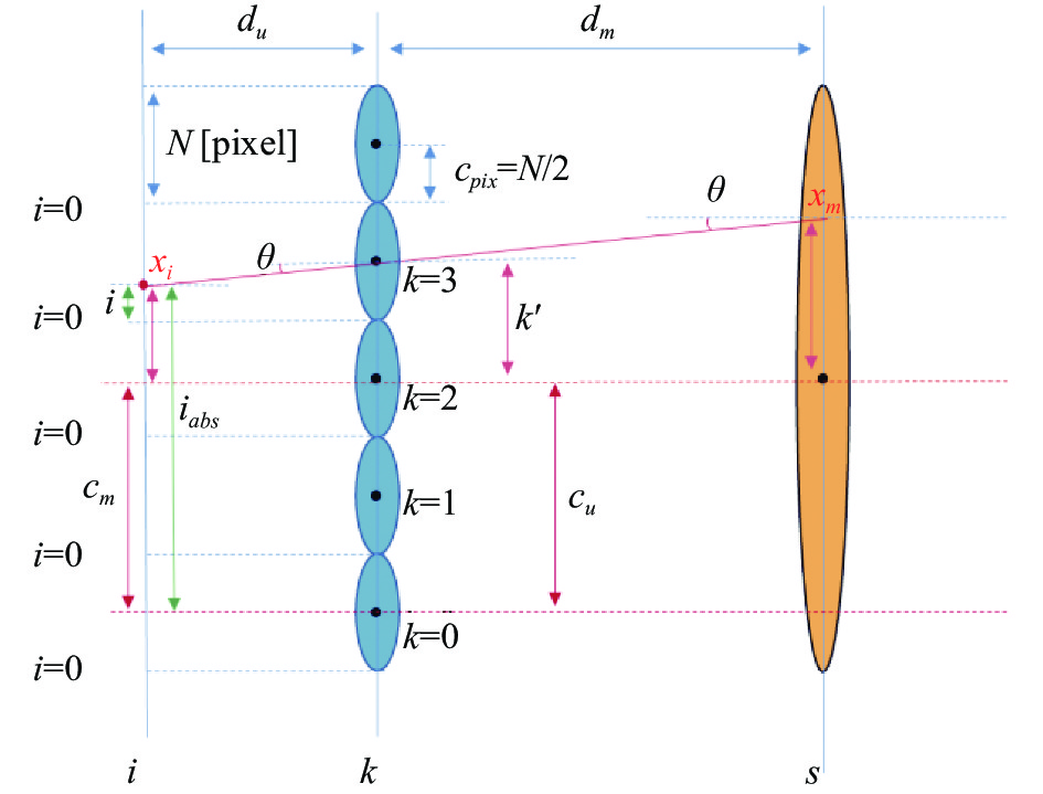
然后通过$H_\varphi ^{{\varPhi }}$推导出其对应光线的角度$\theta $，如图3所示，使用宏像素的中心偏移${c_{pix}}$减去在该宏像素的相对坐标$i$，得到$i$与当前微透镜光轴的像素，然后除以${F_s}$得到该距离的实际物理尺寸$ {x_i} $，最后除以图像传感器平面和微透镜阵列平面的距离$ {d_u} $，即可得到该条光线的角度$\theta $。转换过程如公式(5)所示：$ {x_i} $是光线在图像传感器平面的坐标，$\theta $是光线的角度，$ {d_u} $代表图像传感器平面和微透镜阵列平面的距离。最后通过$ {H^T} $将光线在图像传感器平面的坐标（即光线在${{i}}$平面的坐标$ {x_i} $）延伸至主透镜$ s $平面，如图3所示，主透镜与图像传感器平面的距离($ {d_u} + {d_m} $)乘上光线的角度$\theta $，再加上$ {x_i} $即可得到延伸至主透镜上的点$ {x_m} $，转换过程如公式（6）所示：$ {d_m}$代表主透镜平面与微透镜阵列平面的距离，$ {x_m} $是光线在主透镜$ s $平面的坐标。

最后通过$ {H^M} $推导出入射光线的方向，如图4所示，主透镜符合薄透镜模型，根据高斯成像公式：$ 1/{f_M} = 1/u + 1/v $,$ {f_M} $为主透镜的焦距，$ u $为物距，$ v $为像距，$u = {x_m}/{\theta '}$，$ v = {x_m}/\theta $，即$1/{f_M} = {\theta '}/{x_m} + \theta /{x_m}$，可得到入射光线的角度${\theta '}$，转换过程如公式（7）所示。然后通过$H_{{\varPhi }}^\varphi$推导出经过$ {x_m} $的入射光线与$ u $平面的交点，$ D $是$ u $平面与主透镜$ s $平面的距离，入射光线的角度${\theta '}$与距离$ D $相乘并加上$ {x_m} $即可得到该光线与$ u $平面的交点$ s $，如公式（8）所示：$ s $为入射光线在$ u $平面的坐标，$ u $为入射光线的角度。注意，此时$ u $不是双平面模型中的坐标，而是入射角度，此处是为了和Dansereau等提出的经典模型中的$ u $做区分。

Figure 4.  Light path in the light field camera model

因为垂直和水平方向的索引部分是独立的，所以将2D索引延伸为4D索引是简单的。通过公式（1）将公式（2）中的矩阵相乘可以得到一个具有12个非零项的矩阵的表达式：

微透镜阵列和主透镜都有可能导致镜头畸变^[15]，忽略微透镜阵列产生的畸变，考虑主透镜产生的畸变。由透镜的形状引起的径向畸变模型如下：

式中：$ {k_1} $、$  {k}_{2} $等是径向畸变系数，根据光场相机的镜头参数，可以选择双参数模型和三参数模型；$ u $、$ v $和$ {u_d} $、$ {v_d} $分别为没有畸变和有畸变的光线角度。由相机组装过程中透镜和像面不严格平行引起的切向畸变模型可用畸变系数$ {p_1} $和$ {p_2} $类似描述为：

光场相机的标定有三个主要模块：第一部分是合成所有角度的子孔径图像并提取所有角度子孔径图像的特征点；第二部分是对相机参数进行初始化^[16]；第三部分根据相机的重投影误差构造函数进行非线性优化，它优化了第二部分产生的初始估计。

首先将原始的2D图片解码为4D光场表示，通过得到的微透镜图像合成不同方向的子孔径图像，再对所有子孔径图像进行特征点提取。将每个微透镜宏像素上相同位置的像素点按照顺序进行重排列操作，即可得到该方向的子孔径图像，以此类推，可以得到所有角度的子孔径图像，原理如图5（a）所示。$ i $、$ j $是一个微透镜下的宏像素索引，$ k $、$ l $是微透镜的个数索引。例如：微透镜阵列有$ 381 \times 383 $个，即有$ 381 \times 383 $个微透镜，每个微透镜下的宏像素有 9 pixel×9 pixel，那么就可以提取$ 9 \times 9 $张子孔径图像，每张子孔径图像有381 pixel×383 pixel^[17]。对于子孔径图像来说，$ i $、$ j $是图片索引，$ k $、$ l $是像素值。中心角度的子孔径图像就是按照顺序提取每一个微透镜宏像素中心位置的像素点，然后把这些像素按顺序重新拼接成的图像，所有角度子孔径图像如图5（c）所示，因为每个微透镜的边缘存在渐晕现象，所以边缘角度的子孔径图像较暗。

与传统相机标定类似，光场相机从不同角度拍摄棋盘格图像^[18]，得到所有角度子孔径图像后对子孔径图像进行灰度化处理，然后通过Harris角点检测^[5]方法提取每一幅子孔径图像的特征点。

Figure 5.  Sub-aperture image representation. (a) Sub-aperture image representation of one angle of a given viewpoint; (b) Original light field image; (c) Sub-aperture image of all angles

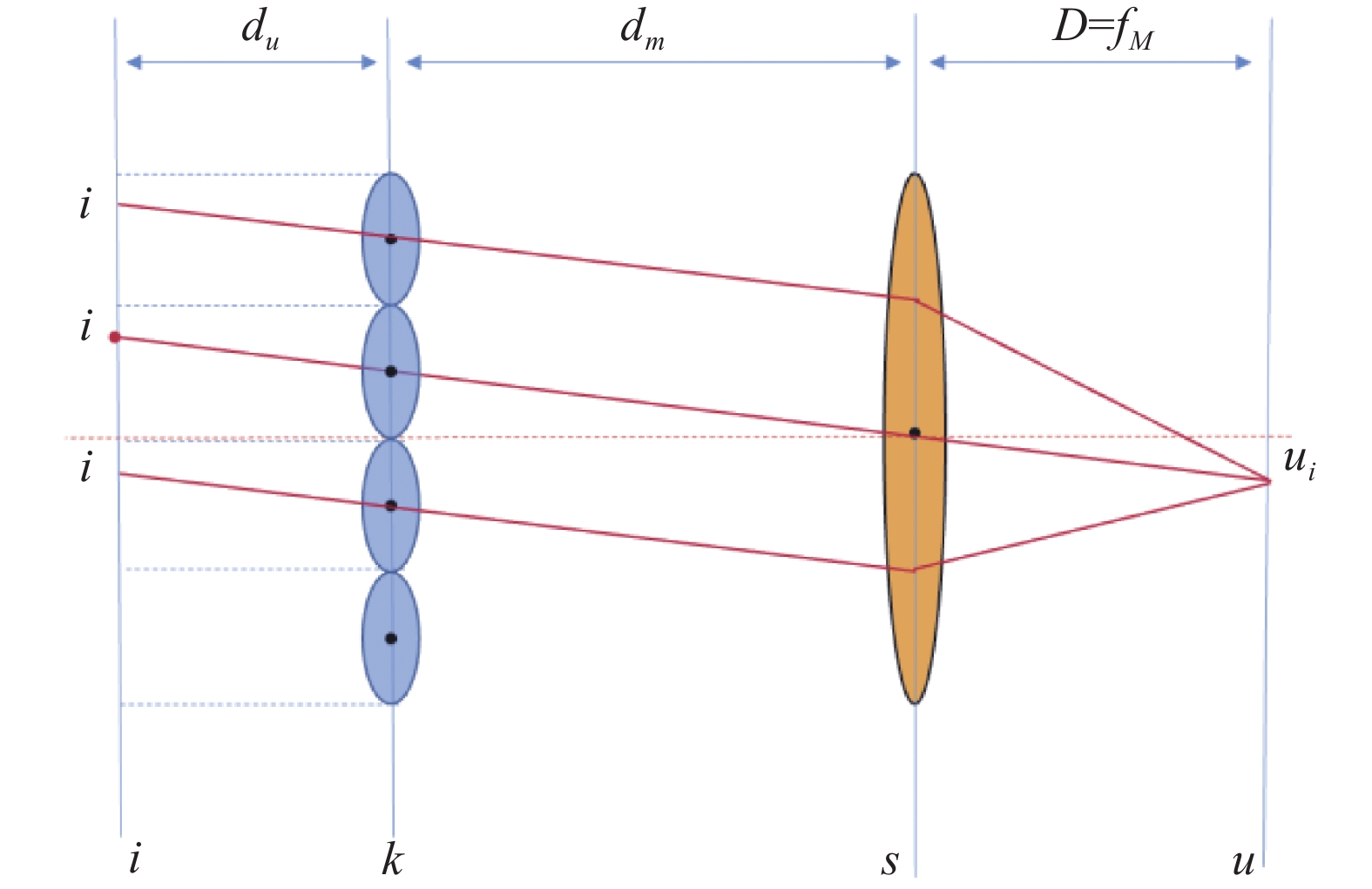
在光场相机的模型中，当$ u $平面在主透镜的焦平面上时，即$ D = {f_M} $，光场相机的坐标系原点为主透镜光轴与主透镜焦平面的交点。$ XY $轴方向仍是像平面的$ XY $方向，$ Z $方向垂直于焦平面向外。通过公式（9）可以得出：$ {H_{1,1}} = {H_{2,2}} $，$ {H_{3,3}} = {H_{4,4}} $，$ {H_{1,3}} = {H_{2,4}} $，$ {H_{3,1}} = {H_{4,2}} $，$ {H_{1,5}} = {H_{{\text{2}},5}} $，$ {H_{{\text{3}},5}} = {H_{4,5}} $。对其参数进行化简，可以得出：$ {H_{1,1}} = - \dfrac{{{f_M}}}{{N{F_u}{d_u}}} $，${H}_{3,3}=-\dfrac{1}{{F}_{\text{u}}{f}_{M}}$，${H_{1,5}} = \dfrac{{{c_{{{pix}}}}{f_M}}}{{N{F_u}{d_u}}}$，$ {H_{{\text{3}},5}} = \dfrac{{{c_u}}}{{{F_u}{f_M}}} $，$ {H_{1,3}} = 0 $，$ {H_{3,1}} = 0 $。

光场相机的初始化首先要得到主透镜的焦距，在光场相机的模型中，从图像传感器到微透镜的每条相同角度的射线路径（即$ i $，$ j $相同）都收敛到主透镜焦平面上的一个点，这个点是虚拟相机的中心位置，即$ {u_i} $，如图6所示。此时，每个子孔径图像的成像等效为小孔成像模型，其焦距是主透镜的焦距$ {f_m} $，子孔径图像相邻像素之间的距离也就是微透镜的物理尺寸，为$ 1/{F}_{u} $ （mm）。中心角度的子孔径图像（光线角度为0°，即过主透镜光心）所等效的虚拟相机的坐标系为光场相机的坐标系。

Figure 6.  Virtual camera center position

类似张正友的平面靶标标定方法^[14]，求解主透镜焦距首先要通过世界坐标系的$3 {\rm{D}}$点和像素坐标系的$2 {\rm{D}}$点得到单应矩阵H：

式中：$ s $表示尺度因子；$ K $表示相机内参矩阵；$ {r_1} $，$ {r_2} $，$ t $为相机外参；$ {f_x} $，$ {f_y} $为主透镜的等效焦距；$ {u_0} $,$ {v_0} $为图像的主点，是两个坐标轴的偏斜参数，可以忽略不计。通过将单应矩阵$ H $中无关的参数（即主点$ ({u_0},{v_0}) $）消除，可以求出焦距$ {f_x} $，$ {f_y} $：

把公式（14）进一步变换，得到：

因为相机外参的旋转矩阵是正交的，即$ {r_1} $和$ {r_2} $正交，由此可推出相机主透镜的等效焦距$ {f_x} $和$ {f_y} $，由$\dfrac{{{h_{11}}{h_{21}}}}{{f_x^2}} + \dfrac{{{h_{12}}{h_{22}}}}{{f_y^2}} + {h_{13}}{h_{23}} = 0$，$ {f_x} = {f_y} $可求得：

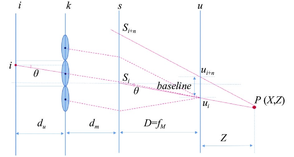
等效焦距等于焦距$ {f_M} $除以像素之间的物理尺寸$ 1/{F_u} $，即$ {f_x} = {f_y} = {f_M}{F_u} $。

相邻虚拟相机中心之间的距离称为基线(baseline)，该基线距可以通过标定时虚拟相机的外参得到，即外参平移量之间的距离，如图7所示。当$ D = {f_M} $时，由图7根据相似三角形可知两个角度$ \theta $是相等的，即：

假如$ n = 1 $，那么基线就是$ {u_{i + 1}} $和$ {u_i} $之间的距离。即通过公式（18）可以得出：

Figure 7.  Light rays from one point to two sub-aperture images at different angles

因此，${H}_{3,3}=-\dfrac{1}{{F}_{{u}}{f}_{M}}=-\dfrac{1}{{f}_{x}}$可以通过公式（17）得到，$ {H_{1,1}} = - \dfrac{{{f_M}}}{{N{F_u}{d_u}}} $可以通过公式（19）得到， ${H}_{1,5}=\dfrac{{c}_{{pix}}{f}_{M}}{N{F}_{u}{d}_{u}}= -{c}_{pix}{H}_{1,1}$，$ {H_{{\text{3}},5}} = \dfrac{{{c_u}}}{{{F_u}{f_M}}} = - {c_u}{H_{3,3}} $。至此，忽略畸变，得到了所有模型参数的初值。

对于传统相机的标定，特征点$ P $对应于图像平面中的某一点，如图8（a）所示，从观测到的和预期得到的投影特征位置$ i $和$ \hat i $之间的距离称为“重投影误差”，$ \left| E \right| = \left| {i - \hat i} \right| $，对这个误差建立目标函数，采用非线性优化方法对相机参数进行优化。但是在光场相机标定中，由于一个特征点会多次出现在成像平面上，重投影误差是比较复杂的，如图8（b）所示，对于光场相机，每个特征点都有多个预期和观测到的图像点$ {\hat i _j} $，$ {i_j} $，并且它们通常不会出现在相同的微透镜下的宏像素内。从每一个观测到的点$ {i_j} $可以得到一条投影光线$ {\phi _j} $，每条投影光线与特征点之间的距离$ \left| {{E_j}} \right| $称为“光线重投影误差”。

Figure 8.  Reprojection error model. (a) Conventional camera projection error; (b) Light field camera projection error

因为已经得到了$ {N_i} \times {N_j} $的子孔径图像阵列，从其中提取观察到的特征点，从$ M $个不同的角度捕获标定板，并且每一个标定板有$ {N_c} $个标定特征点，所以优化的总特征集大小为$ {N_c}M{N_i}{N_j} $。优化目标是找到内参矩阵$ H $、相机姿态$ {T_m} $（光场相机的外参等于最中心的虚拟相机的外参）、畸变系数$ d $、$n = {\left[ {i{\text{ }}j{\text{ }}k{\text{ }}l} \right]^{\rm{T}}}$，$ i $和$ j $为每个微透镜对应像元的索引，即子孔径图像的索引（$ 0 - {N_i} $，$ 0 - {N_j} $），$ k $和$ l $为微透镜的位置索引，即子孔径图像上像素值。$ \phi $表示点$ n $通过畸变校正后通过光场相机模型（公式(1)）得到光线的位置和角度，优化函数如公式（20）所示：

式中：$ {\left\| \cdot \right\|^{pt - ray}} $为“光线重投影误差”。

对该误差建立目标函数，采用 Levenberg-Marquardt的优化算法对其进行优化，使用$ {\text{lsqnonlin}} $函数得到优化后的结果。

利用光场相机Lytro Illum对该方法进行验证。进行标定的实验系统如图9所示，包括光场相机和标定板。从图像传感器上记录的原始$2 {\rm{D}}$图像中恢复$4 {\rm{D}}$光场$ L(s,t,u,v) $，并使用MATLAB toolbox LFToolbox V0.4^[9]进行子孔径图像的提取。使用了相机提供的白图像来定位微透镜图像中心和矫正镜头的渐晕。提取到的四维光场有$ 15 \times 15 $个子孔径图像，每个子孔径图像有434 pixel×625 pixel。实验中，使用Lytro光场相机拍摄16个不同视角的棋盘格图片，该棋盘格有$ 12 \times 9 $个网格，标定板相邻特征点之间的距离为30.0 mm×30.0 mm。

Figure 9.  Light field camera calibration experiment system

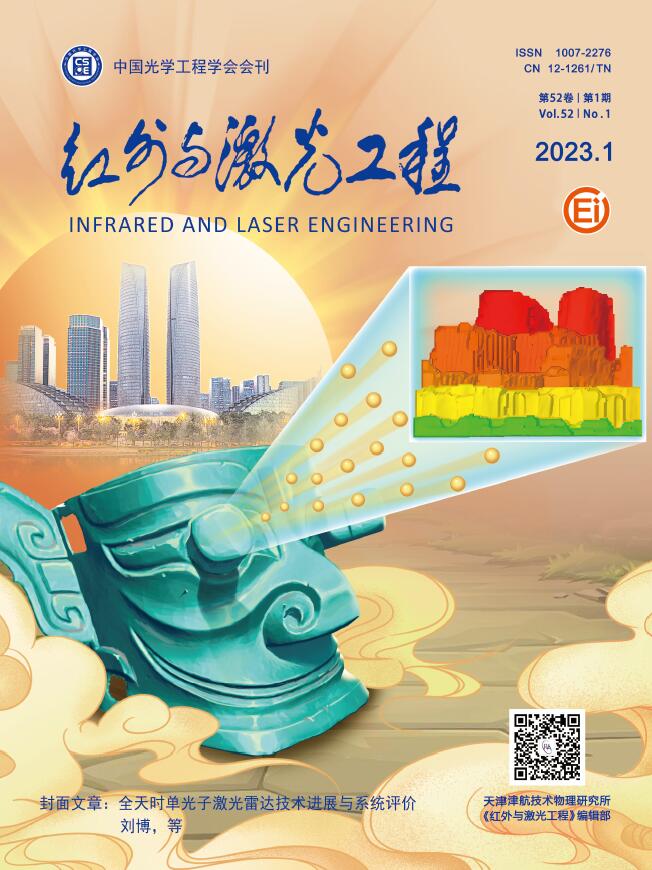
光场相机标定结果详见表1。该模型在非线性优化和畸变校正前后的重投影误差如图10所示。图10(a)中，主透镜边缘的重投影误差相比主透镜中间的重投影误差有较大浮动，而优化校正后的重投影误差大致相同，如图10(b)所示。文中改进的标定方法与Dansereau^[9]等人的方法相比，均方根误差由0.363 mm降低到0.332 mm，精度提升$ 8 \text{%} $，如图10（b）、（c）所示。另外，对于Dansereau^[9]等人方法中采用的径向畸变模型，文中验证了采用多项式模型中双参数、单参数径向畸变模型以及除法模型，其标定精度不如三参数的径向畸变模型，也说明了原本径向模型的准确性。

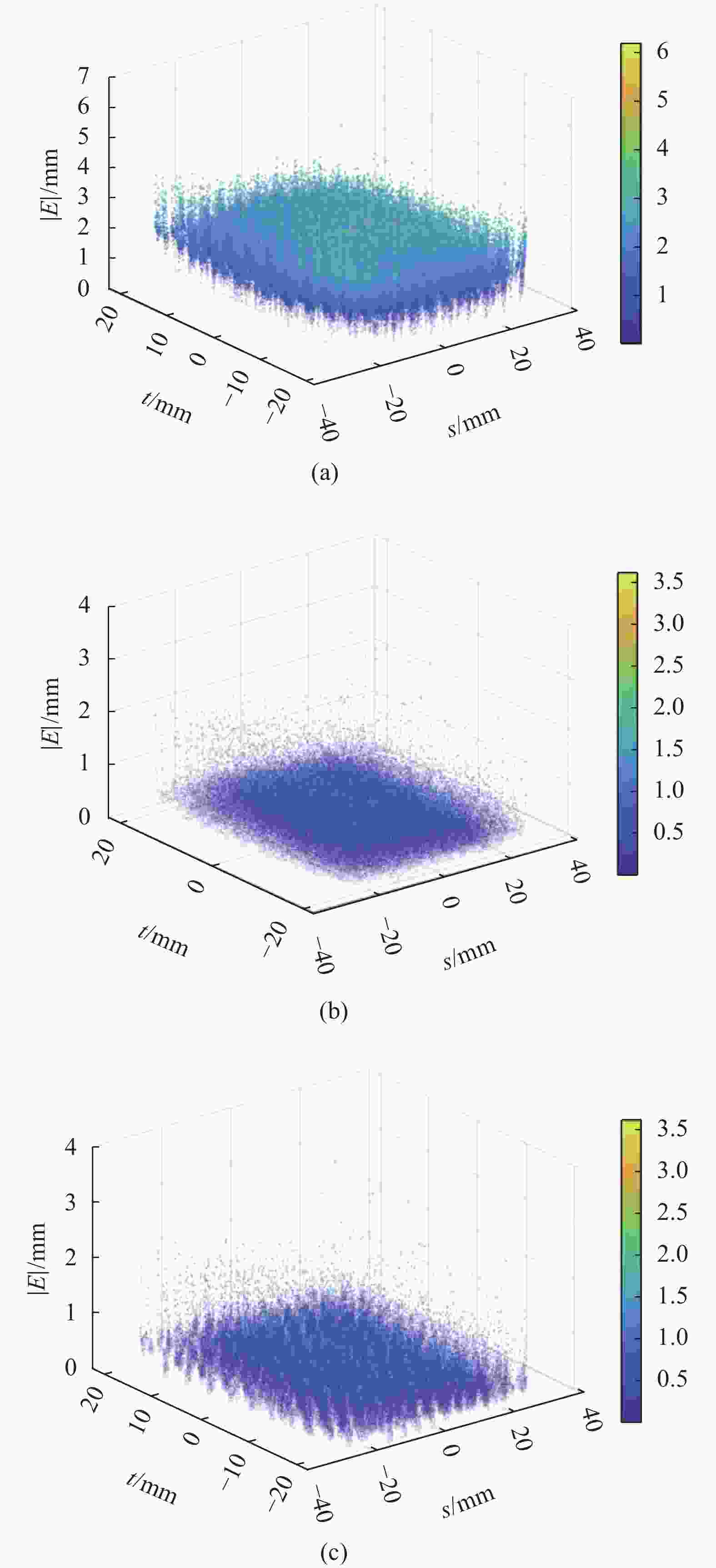
Figure 10.  Reprojection error of 30.0 mm calibration board checkerboard. (a) No nonlinear optimization and distortion correction; (b) Nonlinear optimization distortion correction; (c) The method of Dansereau nonlinear optimization and distortion correction

文中改进了一种双平面模型的光场相机的标定模型和方法。基于微透镜阵列和主透镜模型推导了从场景点到特定像素索引的投影关系，并应用了主透镜的径向和切向畸变校正方法和基于射线重投影的非线性优化方法，实验显示该方法的RMS射线重投影误差为0.332 mm。$ \mathrm{D}\mathrm{a}\mathrm{n}\mathrm{s}\mathrm{e}\mathrm{r}\mathrm{e}\mathrm{a}\mathrm{u} $等人提出的参数模型缺乏对参数的实际物理意义的解释，文中从小孔成像模型和薄透镜模型出发，详细解释了每个参数的物理意义及初值的确定过程，为光场相机模型参数的理解与初始化奠定了理论基础，并且优化了针对光场相机主透镜的畸变模型。下一步计划包括研究一个更复杂的透镜畸变模型以及更精巧的相机投影模型，提高光场标定的准确性，并克服针孔模型和薄透镜模型的局限性。