


 下载:
下载:


-
自由空间光通信(Free Space Optical communication,FSO),是以光为载波、自由空间为传输介质的通信技术,具有传输速率高、通信容量大、光束方向性好和保密性强等优点 [1−3] 。随着无线设备数量的激增,对无线安全性的关注也越来越高。在面对海量数据挑战和信息泄露风险时,确保机密信息传输不受恶意窃听是至关重要的。在采用对称加密技术的情况下,通信双方必须共享密钥以确保安全通信[4]。为了解决密钥共享的挑战,基于信道的密钥提取技术应运而生。这种技术将互易随机信道视为公共随机源,并从中生成共享密钥。通常,无线射频信道被视为常见的随机源[4−6],但近年来,利用大气光信道作为随机源生成密钥也引起了广泛关注[7−9]。大气光信道密钥提取是指使用经典光学技术,对大气光传输信道中的光信号进行密钥提取的过程,并不涉及到量子叠加和纠缠等特殊量子效应,因此不属于量子通信的范畴。在从大气光信道中提取密钥时,首要步骤是在通信两端的合法方对接收到的随机衰落光信号进行采样和测量,从而获得一系列光信号测量样本。随后,这些样本需要经过量化处理,以生成随机比特序列。值得注意的是,测量样本的随机性对最终随机比特序列的质量和安全性会产生影响[10-11]。为了保证从大气光信道中提取的密钥比特的随机性和不确定性,需要根据信道的相关时间将信道状态的测量速率降低到合适的值,以保证连续信道测量之间的不相关性,这一要求对每秒提取的密钥位数施加了限制。对于大气光信道来说,连续的接收光信号测量样本之间存在统计相关的根本原因是,连续的接收光信号测量样本之间缺少随机变化。
为了打破这一限制,文献[12-13]在执行预处理操作来对信道测量样本进行去相关,然后分别对每个去相关条目进行标量量化;这种方法在去相关信道测量方面是有效的,但是需要评估信道估计向量的协方差矩阵及其奇异值分解(SVD),一定程度上依赖于算法的复杂程度。文献[14]针对时分双工单输入单输出(TDD-SISO)系统,设计出了一种基于双向随机性的新型密钥生成(SKG)方法。文献[15]推导了合法通信双方对收发信号施加具备乘性因子的信号,并经过具有互易性的公共信道。理论分析其密钥生成速率上下界。文献[16]提出了一种具有已知人工干扰的密钥生成协议,称为 SmokeGrenade,利用人工干扰来影响信道状态测量值的变化,使得密钥生成率随着干扰功率的增加而增加。若能够设计一种有效的方法,使得发射的光信号在大气湍流光信号衰落自相关时间内能够快速实现随机变化,在采样间隔很小的情况下,可以获得更多更有优势的光信道测量样本,将对整个密钥生成过程产生积极影响。
文献[17]提出对收发两端施加一种随机信号,构建出一种更有优势的带记忆的可控公共随机源(CCRSM),这种创新的方法为实现光信道测量样本去相关,提高密钥生成效率提供了一种新思路。文中在此基础上首先对随机调制实现测量样本去相关性进行了理论分析;基于相关的原理,搭建了基于随机调制实现测量样本去相关的仿真系统,进行数据采集。最后分析了施加随机调制后,对光信道测量样本自相关性的影响。
-
笔者所在课题组前期工作使用共横向空间模式耦合从湍流光无线信道中的信号衰落生成共享密钥的理论分析[7]并搭建了试验系统对大气光信道互易性进行了验证[18]。为了克服湍流本身对于光信道测量样本数量的限制,提出了一种方法,在大气湍流光信号衰落自相关时间内对信道的发射光信号强度进行随机调制,使得发射光信号在大气光信道功率传输系数自相关时间内能够快速随机变化,则在用比其自相关时间长度更小的采样时间间隔条件下,对连续的接收光信号测量样本之间实现去相关[17]。收发端机原理示意图如图1所示。

图 1 基于随机调制的收发端机原理示意图
Figure 1. Schematic diagram of the transceiver based on random modulation
测量两端分别为Alice和Bob两个合法收发端。发射端光信号LSA、LSB分别从激光器A和激光器B发射出来,经过电光调制器后,调制信号源${x_{\rm{A}}}\left( t \right)$、${x_{\rm{B}}}\left( t \right)$分别调制光信号LSA、LSB,${x_A}\left( t \right)$、${x_B}\left( t \right)$会随着发射时间变化且相互独立,在不同t时刻的取值不同且$0 \leqslant {x_{\rm{A}}}\left( t \right) \leqslant 1,0 \leqslant {x_{\rm{B}}}\left( t \right) \leqslant 1$,同时调制信号源变化的自相关远小于大气湍流光信号衰落的自相关时间并进行存储。通过收发光学系统进行发射进入到互易的大气光信道中,从而被Alice和Bob两个合法接收端接收。
Alice和Bob在t时刻接收到的光信号分别为[17]:
$$ \begin{gathered} {y_{\rm{A}}}\left( t \right) = {s_{\rm{B}}}\left( t \right){x_{\rm{B}}}\left( t \right){h_{\rm{M}}}\left( t \right) \\ {y_{\rm{B}}}\left( t \right) = {s_{\rm{A}}}\left( t \right){x_{\rm{A}}}\left( t \right){h_{\rm{M}}}\left( t \right) \\ \end{gathered} $$ (1) 式中:${y_{\rm{A}}}\left( t \right)$和${y_{\rm{B}}}\left( t \right)$分别表示收发光学系统A和收发光学系统B在t时刻收到的光信号功率;${s_{\rm{A}}}\left( t \right)$和${s_{\rm{B}}}\left( t \right)$分别表示激光器A和激光器B发射的光信号功率;${h_{\rm{M}}}\left( t \right)$表示大气光信道功率传输系数,$0 \leqslant {h_{\rm{M}}}\left( t \right) \leqslant 1$。由于大气光信道具有互易性,在合适的条件下,理论上t时刻从Bob到Alice和从Alice到Bob两传输链路终端的大气光信道功率传输系数是相等的。实际实验中,采取一些合理的系统设计和具有优势的算法优化,相关系数可以保持近似为1[18]。Alice 和 Bob 构建共享的公共随机源变为[17]:
$$ \begin{gathered} {\phi _{\rm{A}}}\left( t \right) = {y_{\rm{A}}}\left( t \right){x_{\rm{A}}}\left( t \right) \\ {\phi _{\rm{B}}}\left( t \right) = {y_{\rm{B}}}\left( t \right){x_{\rm{B}}}\left( t \right) \\ \end{gathered} $$ (2) 调制信号源${x_{\rm{A}}}\left( t \right)$、${x_{\rm{B}}}\left( t \right)$在生成的过程中,在本地服务器已经进行了存储,因此完成这一操作是可行的,同时降低了在网络信道传输过程中泄露的风险。于是,${\phi _{\rm{A}}}\left( t \right)$和${\phi _{\rm{B}}}\left( t \right)$可看作是加入随机调制后的接收光信号。因为大气光信道具有互易性,理论上,在t时刻,${\phi _{\rm{A}}}\left( t \right)$和${\phi _{\rm{B}}}\left( t \right)$的互相关系数等于1。这是针对合法双方两端进行都进行随机调制的情形(之后分析过程中用双调制表示)。
当进行合法双方只有一端进行调制时(之后分析过程中用单调制表示),Alice和Bob在t时刻接收到的光信号分别为:
$$ \begin{gathered} {{\tilde y}_{\rm{A}}}\left( t \right) = {s_{\rm{B}}}\left( t \right){x_{\rm{B}}}\left( t \right){h_{\rm{M}}}\left( t \right) \\ {{\tilde y}_{\rm{B}}}\left( t \right) = {s_{\rm{A}}}\left( t \right){h_{\rm{M}}}\left( t \right) \\ \end{gathered} $$ (3) 此时,Alice 和 Bob 构建共享的公共随机源变为:
$$ \begin{gathered} {{\tilde \phi }_{\rm{A}}}\left( t \right) = {{\tilde y}_{\rm{A}}}\left( t \right) \\ {{\tilde \phi }_{\rm{B}}}\left( t \right) = {{\tilde y}_{\rm{B}}}\left( t \right){x_{\rm{B}}}\left( t \right) \\ \end{gathered} $$ (4) 同理,单调制情形下,${\tilde \phi _{\rm{A}}}\left( t \right)$和${\tilde \phi _{\rm{B}}}\left( t \right)$可看作是加入随机调制后的接收光信号。因为大气光信道具有互易性,理论上,在t时刻 ${\tilde \phi _{\rm{A}}}\left( t \right)$和${\tilde \phi _{\rm{B}}}\left( t \right)$的互相关系数等于1。
-
该节通过时间序列自协方差函数分析调制信号源${x_{\rm{A}}}\left( t \right),{x_{\rm{B}}}\left( t \right)$和大气光信道功率传输系数${h_{\rm{M}}}\left( t \right)$,作用是分析在任意两个不同时刻的取值之间的二阶混合中心矩,描述在两个时刻取值的起伏变化的相关程度。${\phi _{\rm{A}}}\left( t \right),{\phi _{\rm{B}}}\left( t \right)$两次连续观测值的相关系数分别为[17]:
$$ \begin{gathered} {b_{\phi ,{\rm{A}}}}\left( \tau \right) \simeq \frac{{{b_h}\left( \tau \right)}}{{\zeta \left( {{\gamma _{\rm{A}}},\sigma _{x,{\rm{A}}}^2,\sigma _{x,{\rm{B}}}^2} \right)}} \\ {b_{\phi ,{\rm{B}}}}\left( \tau \right) \simeq \frac{{{b_h}\left( \tau \right)}}{{\zeta \left( {{\gamma _{\rm{B}}},\sigma _{x,{\rm{B}}}^2,\sigma _{x,{\rm{A}}}^2} \right)}} \\ \end{gathered} $$ (5) 式中:$\sigma _{x,{\rm{A}}}^2,$$\sigma _{x,{\rm{B}}}^2,$$ \sigma _h^2 $分别代表${x_{\rm{A}}}\left( t \right),$ ${x_{\rm{B}}}\left( t \right),$ ${h_{\rm{M}}}\left( t \right)$的归一化方差反映了信号的波动性的变化;${\gamma }_{{\rm{A}}}和{\gamma }_{{\rm{B}}}$分别是 Alice 和 Bob 光电探测器输出端的平均信噪比 (SNR);${b_h}\left( \tau \right) = \exp \left( { - {\tau ^2}/\tau _{h,0}^2} \right)$,${\tau _{h,0}}$是大气光信道传输系数的相干时间,理论分析过程中令${b_h}\left( \tau \right) = {{\mathrm{e}}^{ - 1}}$。${b_h}\left( \tau \right)$是大气光信道传输系数${h_{\rm{M}}}\left( t \right)$归一化时间自协方差函数。
$$ \begin{gathered} \zeta \left( {{\gamma _{\rm{A}}},\sigma _{x,{\rm{A}}}^2,\sigma _{x,B}^2} \right) = \left( {\sigma _{x,{\rm{A}}}^2 + 1} \right)\left( {\sigma _{x,{\rm{B}}}^2 + 1} \right) + \left[ {\left( {\sigma _{x,{\rm{A}}}^2 + 1} \right)\left( {\sigma _{x,{\rm{B}}}^2 + 1} \right) + \gamma _{\rm{A}}^{ - 1}\left( {\sigma _{x,{\rm{A}}}^2 + 1} \right) - 1} \right]\sigma _h^{ - 2} \\ \zeta \left( {{\gamma _{\rm{B}}},\sigma _{x,{\rm{B}}}^2,\sigma _{x,{\rm{A}}}^2} \right) = \left( {\sigma _{x,{\rm{B}}}^2 + 1} \right)\left( {\sigma _{x,{\rm{A}}}^2 + 1} \right) + \left[ {\left( {\sigma _{x,{\rm{B}}}^2 + 1} \right)\left( {\sigma _{x,{\rm{A}}}^2 + 1} \right) + \gamma _{\rm{B}}^{ - 1}\left( {\sigma _{x,{\rm{B}}}^2 + 1} \right) - 1} \right]\sigma _h^{ - 2} \\ \end{gathered} $$ (6) $\zeta \left( {{\gamma _{\rm{A}}},\sigma _{x,{\rm{A}}}^2,\sigma _{x,{\rm{B}}}^2} \right)$和$\zeta \left( {{\gamma _{\rm{B}}},\sigma _{x,{\rm{B}}}^2,\sigma _{x,{\rm{A}}}^2} \right)$是由${\gamma _{\rm{A}}},$${\gamma _{\rm{B}}},$$\sigma _{x,{\rm{A}}}^2,$$\sigma _{x,{\rm{B}}}^2,$$ \sigma _h^2 $针对$ {b_h}\left( \tau \right) $构建的参数比例因子。调制信号源${x_{\rm{A}}}\left( t \right),{x_{\rm{B}}}\left( t \right)$的归一化方差$\sigma _{x,{\rm{A}}}^2,$$\sigma _{x,{\rm{B}}}^2$分别对于 ${\tilde \phi _{\rm{A}}}\left( t \right)$,${\phi _{\rm{A}}}\left( t \right)$的两次连续观测值的相关系数的影响如图2所示。分析过程中限制${\gamma _{\rm{A}}} \equiv \infty$${\gamma _{\rm{B}}} = \infty$,同时接收信号样本采样间隔时间远小于大气光信道功率传输系数自相关时间。
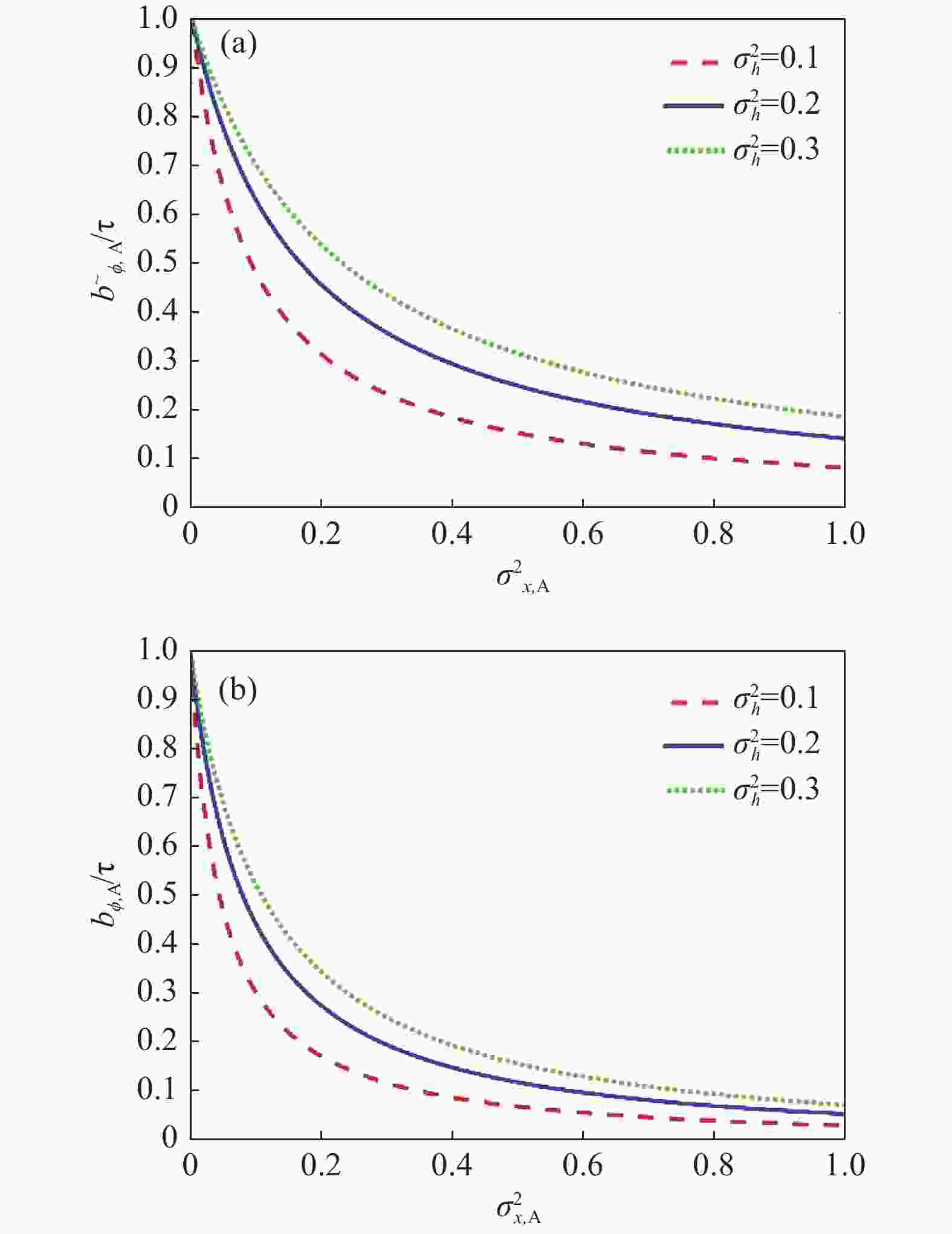
图 2 (a)单调制情况下对${\tilde \phi _{{{\rm{A}}}}}\left( t \right)$两次连续观测值的相关系数分析图,$\sigma _{x,{{{\rm{A}}}}}^2 > 0,\sigma _{x,{{{\rm{B}}}}}^2 \equiv 0$;(b)双调制情况下对${\phi _{\rm{A}}}\left( t \right)$两次连续观测值的相关系数分析图,$\sigma _{x,{{{\rm{A}}}}}^2 \equiv \sigma _{x,{{{\rm{B}}}}}^2 > 0$
Figure 2. (a) Correlation coefficient analysis of two consecutive observations of ${\tilde \phi _{{{\rm{A}}}}}\left( t \right)$ in the case of signal modulation $\sigma _{x,{{{\rm{A}}}}}^2 > 0,\sigma _{x,{{{\rm{B}}}}}^2 \equiv 0$;(b) Correlation coefficient analysis of two consecutive observations of ${\phi _{{{\rm{A}}}}}\left( t \right)$ in the case of double modulation$\sigma _{x,{{{\rm{A}}}}}^2 \equiv \sigma _{x,{{{\rm{B}}}}}^2 > 0$
图2(a)为单调制情况下对${\tilde \phi _{\rm{A}}}(t)$分析图, ${x_{\rm{A}}}(t)$随时间随机变化,$\sigma _{x,{\rm{A}}}^2 > 0$,${x_{\rm{B}}}(t)$不随时间随机变化,$\sigma _{x,{\rm{B}}}^2 = 0$。横坐标为$\sigma _{x,{\rm{A}}}^2$,代表调制信号的波动性变化,纵坐标为${b_{\tilde \phi ,{\rm{A}}}}\left( \tau \right)$,代表单调制情况两次连续观测值的相关系数,反映相邻测量样本的自相关情况。$ \sigma _h^2 $反映大气光信道功率传输系数的波动性变化。图2(b)为双调制情况下对${\phi _{\rm{A}}}(t)$的分析图,${x_{\rm{A}}}(t)$,${x_{\rm{B}}}(t)$都随时间发生变化,$\sigma _{x,{\rm{A}}}^2 = \sigma _{x,{\rm{B}}}^2 > 0$;纵坐标为${b_{\phi ,{\rm{A}}}}\left( \tau \right)$,代表单调制情况两次连续观测值的相关系数,反映相邻测量样本的自相关情况。下面从调制情况、大气光信道功率传输系数的波动性变化情况和调制信号的波动性变化情况三个角度,分析对于相邻测量样本自相关影响。
对于不同的调制情况,对比图2(a)和图2(b)中$\sigma _h^2 = 0.3$曲线可以发现,两种情况下,随着自变量$\sigma _{x,{\rm{A}}}^2$增加,两次连续观测值的相关系数不断降低,双调制情况下相关系数随着$\sigma _{x,{\rm{A}}}^2$增加,下降的更快。同时单调制情况下$\sigma _{x,{\rm{A}}}^2 \equiv 1$时,两次连续观测值的相关系数在0.2附近,而双调制情况下两次连续观测值的相关系数小于0.1,变化幅度更明显。
对于大气光信道功率传输系数的波动性变化情况,通过对比图2(a)中$\sigma _h^2 = 0.3$,$\sigma _h^2 = 0.2$,$\sigma _h^2 = 0.1$,发现随着$\sigma _h^2$减小,大气光信道功率传输系数的单位时间内波动性变化减弱,两次连续观测值的相关系数的下降幅度变得更大。具体来说,当$\sigma _{x,{\rm{A}}}^2 = 1$时,在此条件下,$\sigma _h^2 = 0.3$时的相关系数小于0.2,而$\sigma _h^2 = 0.1$时,相关系数小于0.1,变化幅度更大。分析得出大气光信道功率传输系数的波动性变化对于测量样本的自相关性具有重要影响。
对于调制信号的波动性变化情况,观察图2(a)和图2(b)可以发现,随着 $\sigma _{x,{\rm{A}}}^2$的增加,调制信号单位时间内波动性变化增强,两次连续观测值的相关系数减小。
-
基于随机调制光信道样本测量系统如图3所示,合法方Alice这边的激光器A于发射端发出连续光波,经过电光调制器m1把任意波形发生器(AWG)g1产生的伪随机波动的波形引入到初始传输光信号功率。发射光信号在大气湍流光信号衰落自相关时间内能够快速随机变化,同时在计算机本地进行存储,b1的作用是提供电光调制器偏置电压。经过调制后的光信号经过环形分光器c1,通过光学镜筒a1扩束发射到大气湍流信道中,被合法方Bob端的光学镜筒a1进行收缩接收,再经过环形分光器c2,最终输入到光电探测器d2,光电探测器探测完传输到计算机本地进行存储。Bob端的运行机理与Alice端相似,不同之处在于任意波形发生器(AWG)g2和任意波形发生器(AWG)g1产生的伪随机波动的波形之间是相互独立的。由系统示意图可知,光信号经过两次随机调制的测量样本数据是不能直接进行测得的。此次仿真实验过程中,双调制的数据主要通过任意波形发生器(AWG)在本地服务器存储的数据和探测器(Detector)采集到对方激光随机调制的光信号的实时测量样本数据在计算机本地服务器中点乘计算得出的。
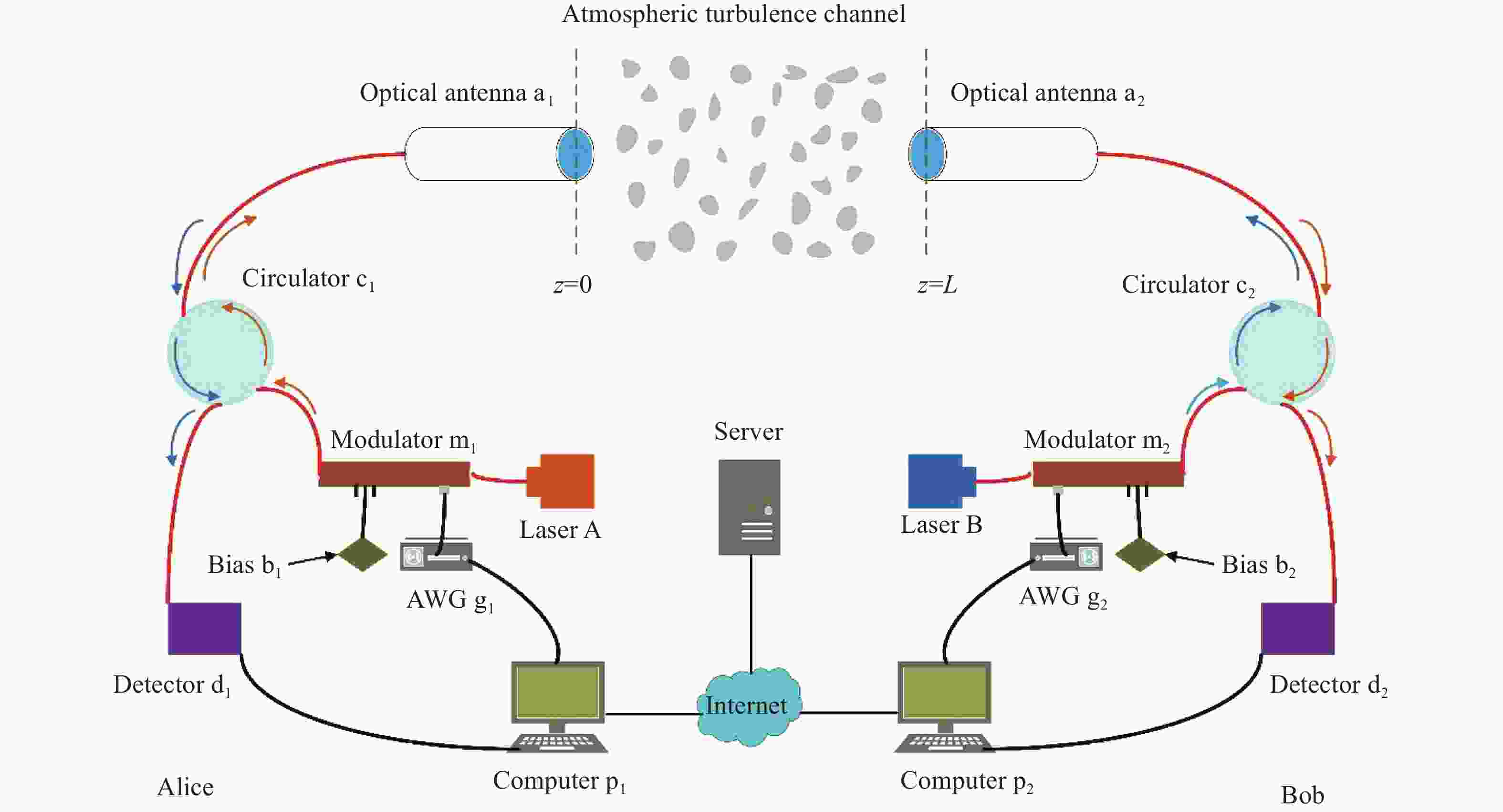
图 3 基于随机调制光信道样本测量系统示意图
Figure 3. Schematic diagram of optical channel sample measurement system based on random modulation
文中针对随机调制对湍流引起的光学波动的相关时间对每秒提取的不相关光信道测量样本的数量限制影响进行了仿真研究。需要构建一个湍流引起的光学波动的相关时间对每秒提取的不相关光信道测量样本的数量造成限制的仿真情境。因此参数设置过程中需要样本的采样间隔时间远小于大气光信道相干时间[17]。仿真研究过程中,伪随机码生成速率是自变量,为了保证生成的伪随机调制信号的稳定性,设置采样时间为$1.28 \times {10^{ - 3}}$ s,样本采样速率为$6.4 \times {10^6}$ Hz。仿真过程中这两个参数是恒定的。样本数量为8 192,是采样时间乘以样本采样速率的计算结果。仿真过程中,设置的大气光信道相干时间为$0.4 \times {10^{ - 4}}$ s。大气光信道相干时间和采样时间存在比例关系1∶32,或者说在采样时间内波动变化32次。同时为了分析调制信号对于测量样本自相关性的影响,调制信号单位时间内波动变化程度需要大于大气光信道传输系数相干时间波动变化程度[17]。当伪随机码生成速率为105 bit/s时,调制信号单位时间内波动变化程度和大气光信道传输系数相干时间波动变化程度的比例为1∶1.75 ~ 1∶2。此时采集到的功率随时间变化的图效果比较好。仿真过程中信道参数设置为大气折射率结构常数,选择的是$C_n^2 = 5 \times {10^{ - 15}}{m^{ - 2/3}}$,传输距离为1 km,衰减为20 dB/km,仿真结果适用于中湍流的条件[19]。
利用Optisystem软件仿真研究过程中,Alice和Bob两个合法端激光器为CW Laser;任意波形发生器(AWG)的仿真测试装置为Pseudo-Random Sequence Generator,主要调节设置的参数为比特生成速率。生成的伪随机码电信号波形由仿真测试装置中内置的Oscilloscope Visualier测量和显示。主要分析生成电信号的振幅和时间关系。通过FSO中FSO channel用于模拟光通信或光传感系统中的大气传输介质,主要调节设置的参数为光强闪烁的相干时间。光信号的功率采集主要通过软件中内置的光时域可视分析仪(Optical Time Domain Visualizer )进行测量和显示。
-
基于随机调制光信道样本测量仿真系统,研究了不同调制情况、不同大气光信道传输系数相干时间、不同伪随机码生成速率、传输距离以及信噪比对光信道测量样本自相关性的影响。
-
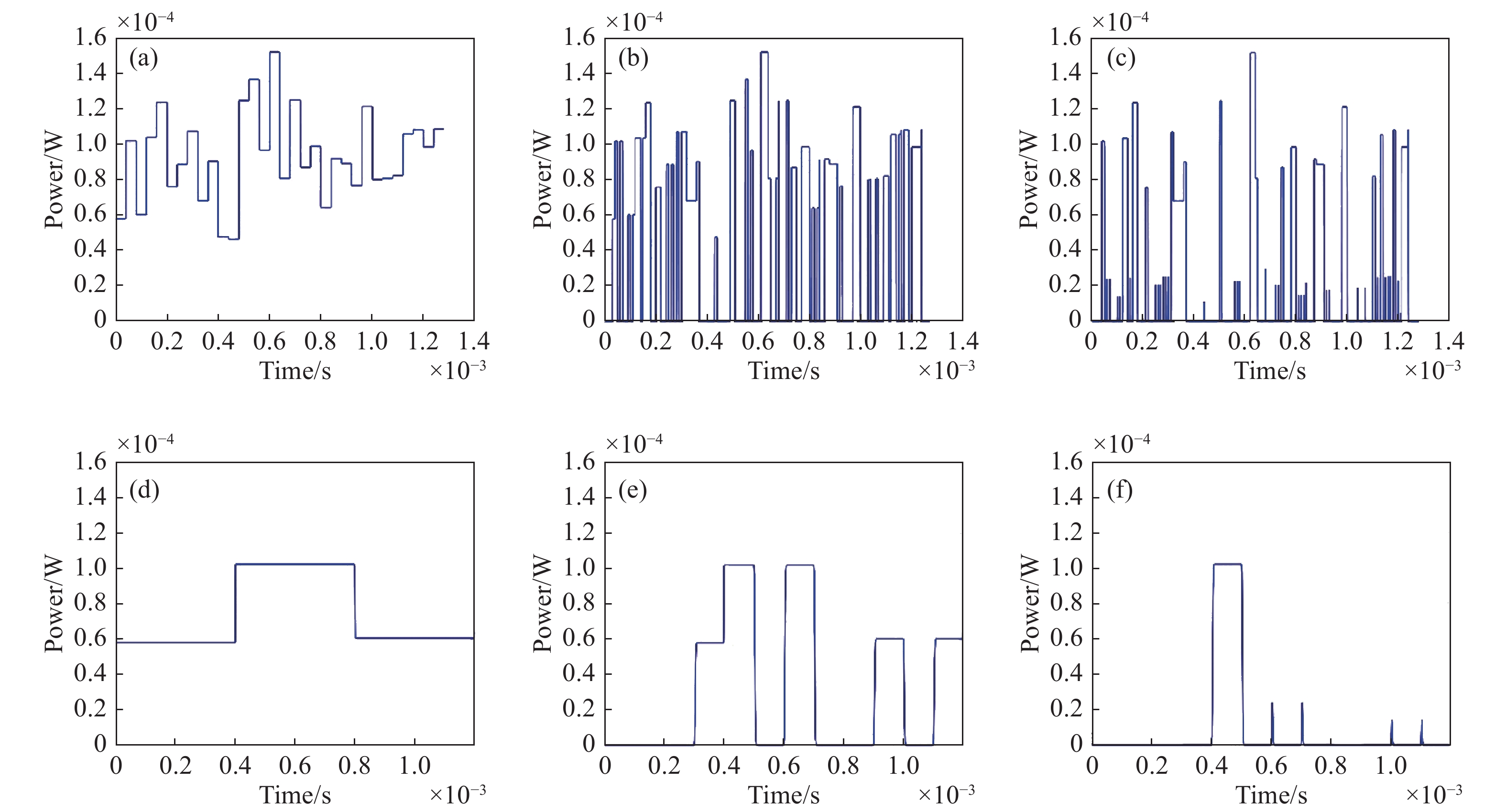
该小节描述的是无调制、单调制和双调制三种情况下,分析基于随机幅度调制的连续激光信号,在大气光信道中,沿水平传输路径的光信道测量样本去相关性分析。仿真研究过程中使用的基本参数为:激光波长为1 064 nm,功率为30 dBm,传输距离为1 km,信道衰减系数为20 dB/km,信道相干时间为$0.4 \times {10^{ - 4}}$ s,大气折射率结构常数选择的是$C_n^2 = 5 \times {10^{ - 15}}\;{{\rm{m}}^{ - 2/3}}$,收发端望远镜接收孔径为8 cm,采样速率为$6.4 \times {10^6}$ Hz,采样时间为$1.28 \times {10^{ - 3}}$ s,伪随机码生成速率为${10^5}$ bit/s。仿真研究过程中,分析不同情况时,会对变量参数进行说明,如无特殊说明仿真参数均为以上参数。图4(a)~4(c)是8 192个光信号测量样本在不同调制情况下功率随时间变化图像。观察图4(a)~图4(c)可以发现在无调制、采样速率很快的情况下,采集到的光信号测量样本缺乏随机变化,而在单调制和双调制情况下这一现象有了一定程度的改善。
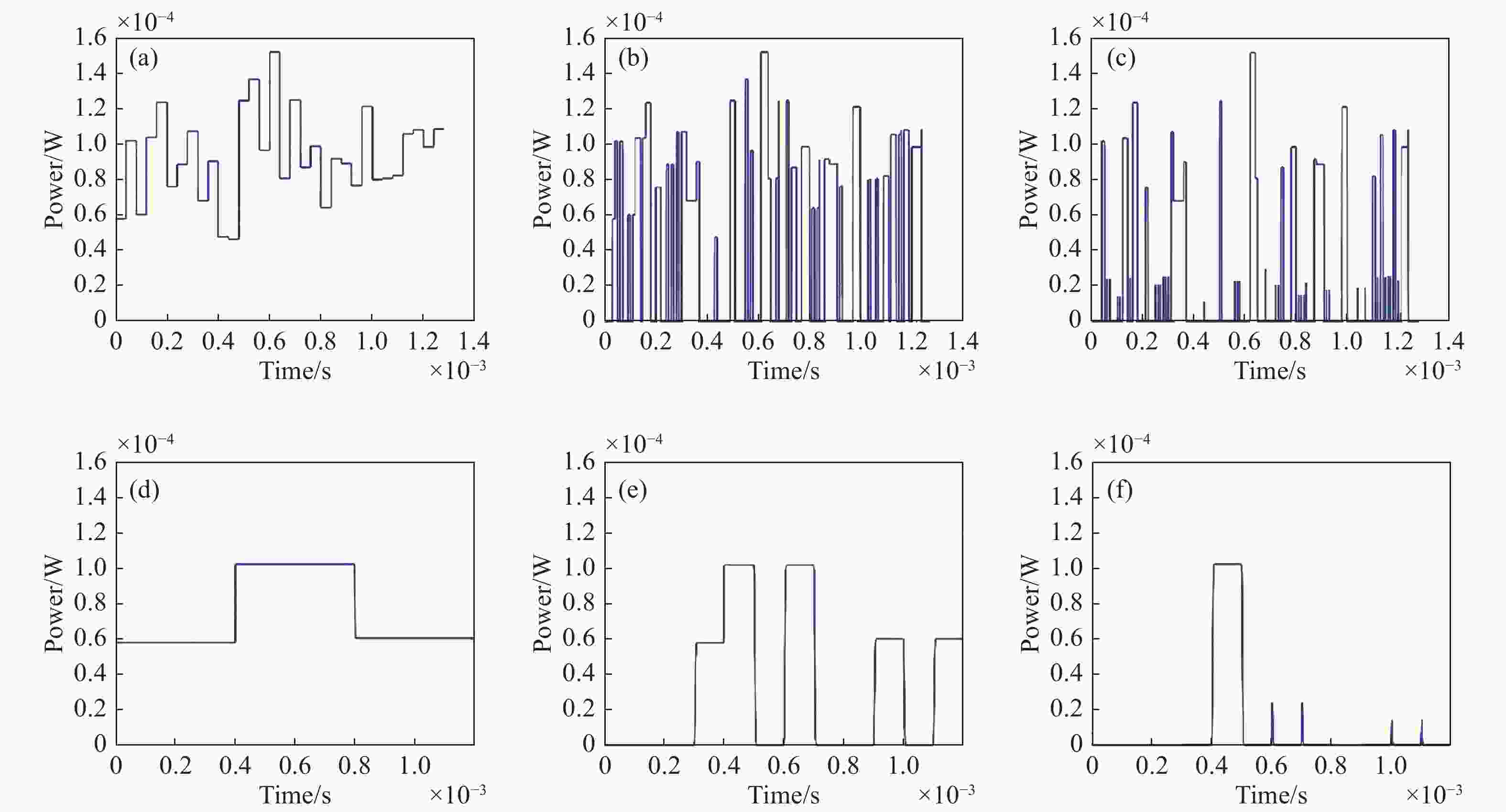
图 4 (a)无调制情况下实时测量数据图;(b)单调制情况下实时测量数据图;(c)双调制情况下实时测量数据图;(d)、(e)和(f)分别为不同调制情况下 0 ~ 0.119 × 10⁻³ s测量数据图
Figure 4. (a) Real-time measurement data plot in the case of no modulation; (b) Real-time measurement data plot in the case of single modulation; (c) Real-time measurement data plot in the case of double modulation; (d), (e), and (f) are the 0 -0.119 × 10⁻³ s measurement data plots in different modulation cases, respectively
为了更为具体的分析,截取了不同调制情况下在0 ~ 0.119 × 10⁻³ s之间采集的功率信号和时间的波形,生成图4(d)~4(f)。通过 对比分析,由图4(d)可知,在无调制的情况下,在0 ~ 0.398 × 10⁻⁴ s之间采集的光信号功率和时间的波形发生了三次变化,在0 ~ 0.389× 10⁻⁴ s之间有256个测量样本功率在0.581 6 × 10⁻⁴波动,0.389 × 10−4 s ~ 0.798 × 10⁻⁴ s之间有256个测量样本功率在1.021 7 × 10⁻⁴ s细微波动,在0.798 × 10⁻⁴ s ~ 0.119 × 10⁻³ s之间有256个测量样本在0.605 2 × 10⁻⁴细微波动,由于模拟过程中光强闪烁的相干时间是固定的,所以每次变化的测量样本的数量都是256。说明当采样速率远高于大气湍流引起的光功率变化的时间尺度时,采集到的光信号测量样本可能在大部分时间内保持相似,则连续的信道测量不可避免地在统计上相关。这样的测量样本经过特征量化等步骤生成的密钥序列通常没有足够的随机性,甚至可能出现密集的连续0、1 bit。简单来说,这样的密钥序列不满足作为密钥需要的条件。由图4(e)、图4(f)可知,单调制情况下采集的功率信号和时间的波形发生了9次变化,双调制情况下采集的功率信号和时间的波形发生了11次变化。对比无调制情况下在相同时间间隔内,测量样本的变化次数有了明显的提高,得到的光信道测量样本作为密钥的随机源更具有优势。
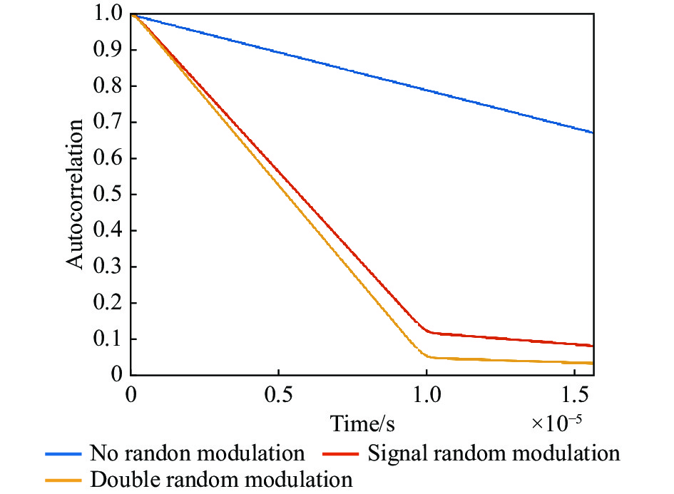
为了分析不同调制情况下光信号测量样本的自相关性,利用数值分析软件中内置的自相关函数对图4(a)~图4(c) 所代表的测量数据进行计算分析并进行归一化处理,分析不同调制情况下测量样本的自相关性。
不同调制情况下自相关性对比分析如图5所示,蓝色线代表的是无调制的情况,红色线代表的是单调制的情况,黄色线代表的是双调制的情况。由图5可知,自相关函数在延迟为0的位置为最大值,代表信号与自身的完全相关性。随着延迟时间的不断增加,测量样本与其自身在不同延迟下的自相关性逐渐衰减。无随机调制情况下,测量样本在不同延迟时间下衰减速度缓慢,滞后100个样本后自相关性为0.676。对比发现,单调制情况下和双调制情况下,随着延迟时间的增加,测量样本衰减速度明显提高。相同情况下,不同延迟时间下的测量样本的自相关性显著降低,滞后100个样本后自相关性分别为0.083和0.035。一定程度上实现了测量样本的去相关。

图 5 不同调制情况下自相关性对比分析图
Figure 5. Comparative analysis of autocorrelation for different modulations
-
针对单调制情况,该小节分析了在其他参数固定,大气光信道传输系数相干时间在$0.1 \times {10^{ - 4}}\;{\mathrm{s}}$,$0.4 \times {10^{ - 4}}\;{\mathrm{s}}$和$0.7 \times {10^{ - 4}}\;{\mathrm{s}}$时,基于随机幅度调制的连续激光信号,在大气光信道中,沿水平传输路径的光信道测量样本去相关性,结果如图6所示。
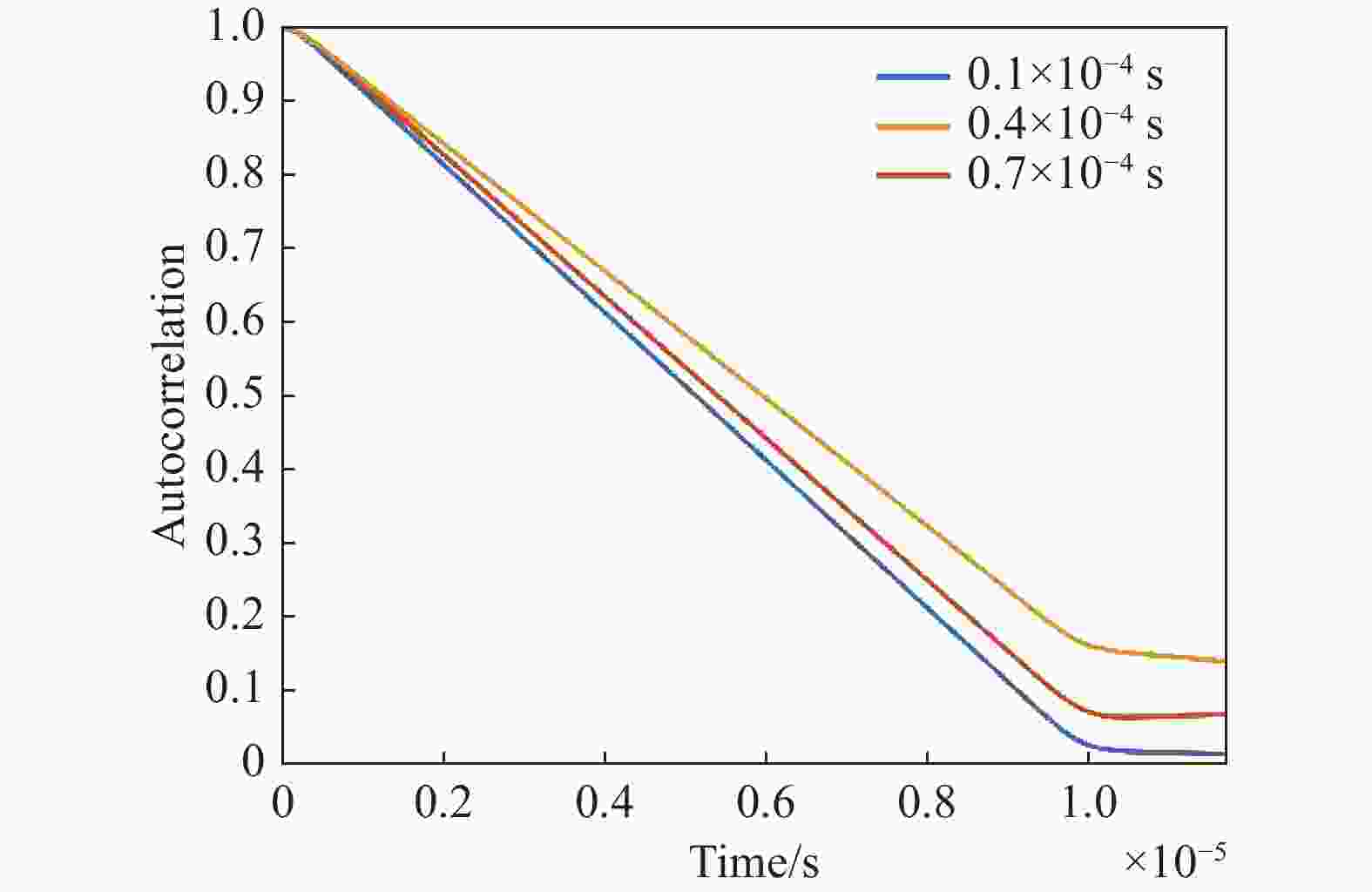
图 6 大气光信道传输系数不同相干时间对比分析图
Figure 6. Comparative analysis diagram of atmospheric optical channel transmission coefficients with different coherence times
由图6可知,在湍流强度、传输距离等参数一定的条件下,大气光信道参数相干时间在$0.1 \times {10^{ - 4}}\;{\mathrm{s}}$,$0.4 \times {10^{ - 4}}\;{\mathrm{s}}$和$0.7 \times {10^{ - 4}}\;{\mathrm{s}}$时,滞后75个测量样本延迟时间后的自相关性分别为0.014、0.069、0.141。对比发现,大气光信道参数${h_{\rm{M}}}\left( t \right)$的相干时间为$0.1 \times {10^{ - 4}}\;{\mathrm{s}}$时,随着延迟时间增加,测量样本的自相关性衰减速度更快,变化幅度更明显。分析得出,随着大气光信道传输系数相干时间减小,延迟时间增加,测量样本的自相关性衰减速度更快,变化幅度更明显。
-
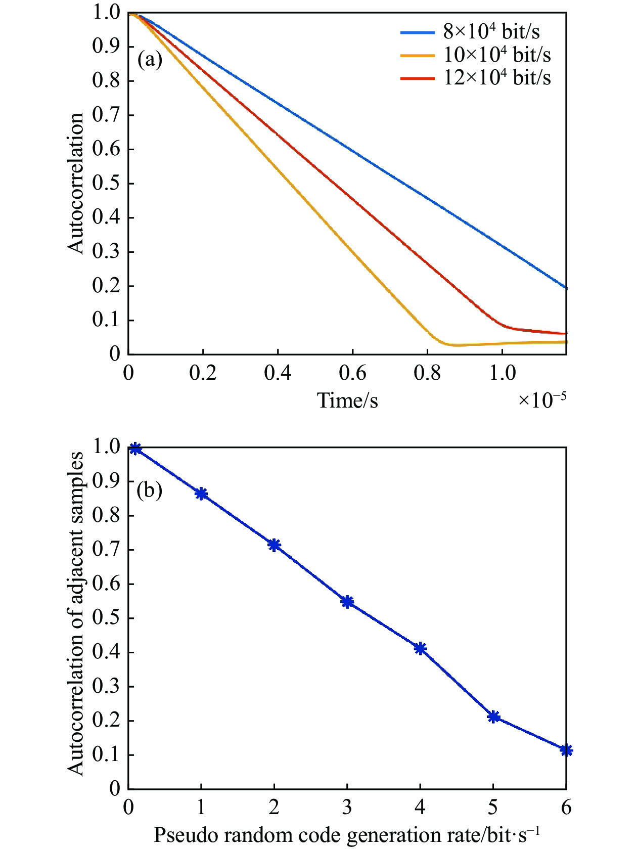
针对单调制情况,该小节分析了在其他参数固定,生成随机调制信号的伪随机码生成速率在$8 \times {10^4}$ bit/s,$10 \times {10^4}$ bit/s和$12 \times {10^4}$ bit/s时,基于随机幅度调制的连续激光信号,在大气光信道中,沿水平传输路径光信道测量样本去相关性,结果如图7(a)所示。同时通过测量在$0 \sim 6 \times {10^6}$ bit/s生成速率的情况下,每隔${10^6}$ bit/s相邻测量样本的自相关性。分析了随着生成随机调制信号的伪随机码生成速率不断提高,随机幅度调制的连续激光信号,对于水平传输情形的大气光信道所采集的相邻测量样本的自相关情况,结果如图7(b)所示。
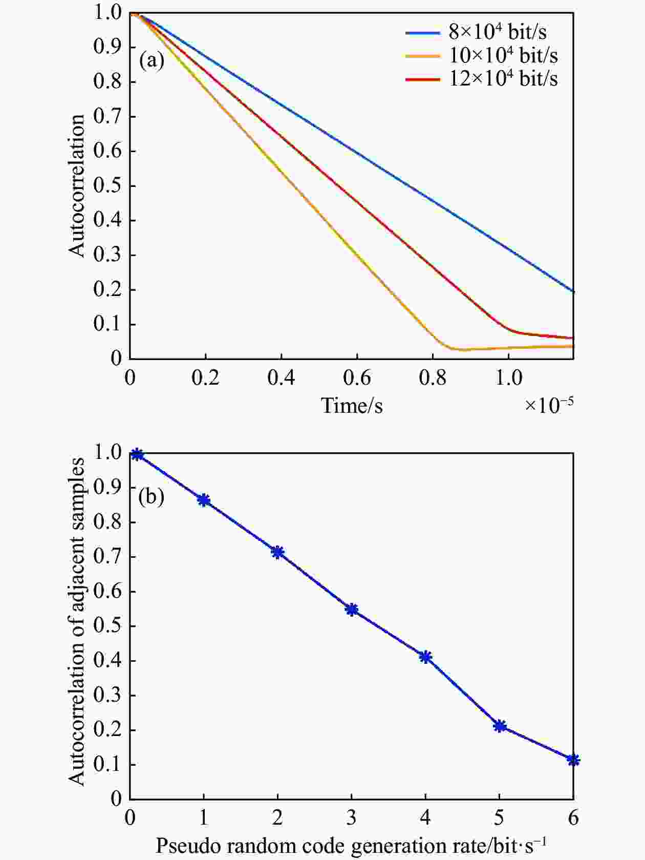
图 7 (a) 伪随机码不同生成速率对比分析图;(b)相邻测量样本自相关分析图
Figure 7. (a) Comparative analysis diagram of pseudo random code with different generation rates; (b)Autocorrelation analysis diagram of adjacent measurement samples
由图7(a)可知,当湍流强度、传输距离等参数一定条件下,生成随机调制信号的伪随机码生成速率在$8 \times {10^4}$ bit/s,$10 \times {10^4}$ bit/s和$12 \times {10^4}$ bit/s的情况下,滞后75个测量样本延迟时间后的自相关性分别为0.194、0.063、0.033。对比发现,伪随机码的生成速率$12 \times {10^4}$ bit/s的情况下,随着延迟时间增加,测量样本的自相关性衰减速度最快,变化幅度更明显。分析得出,随着伪随机码生速率加快,延迟时间的增加,测量样本的自相关性衰减速度更快,变化幅度更明显。
由图7(b)可知,随着伪随机码生成速率的不断增强,单位时间内调制信号的波动性增强,相邻测量样本自相关性显著减小。当样本采样速率为$6.4 \times {10^6}$ Hz,伪随机码生成速率达到$6 \times {10^6}$ bit/s时,相邻测量样本的自相关性为0.112。结果表明,伪随机码生成速率足够快的情况下,生成的随机调制信号的相关时间远小于大气光信道传输系数相干时间。对发射光信号功率进行随机调制,可以使其在小于湍流引起的光学波动的相关时间的采样间隔下,对于合法观测方观测到的光信道相邻测量样本进行去相关。
-
针对单调制情况,该小节分析了在其他参数固定,连续激光信号在传输距离为$0.5$、$0.8$、1.5 km时,基于随机幅度调制的连续激光信号,在大气光信道中,沿水平传输路径的光信道测量样本去相关性,分析结果如图8所示。

图 8 不同距离情况下自相关性对比分析图
Figure 8. Plot of comparative analysis of autocorrelation at different distances
由图8可知,经过随机调制后,不同距离的光信道测量样本的自相关性随着延迟时间的增加而下降地更快,滞后100个样本后自相关性从$0.6 \sim 0.7$之间降低到0.3以下,变化幅度明显。说明随机调制对不同距离情况下测量样本的自相关性产生了影响。
-
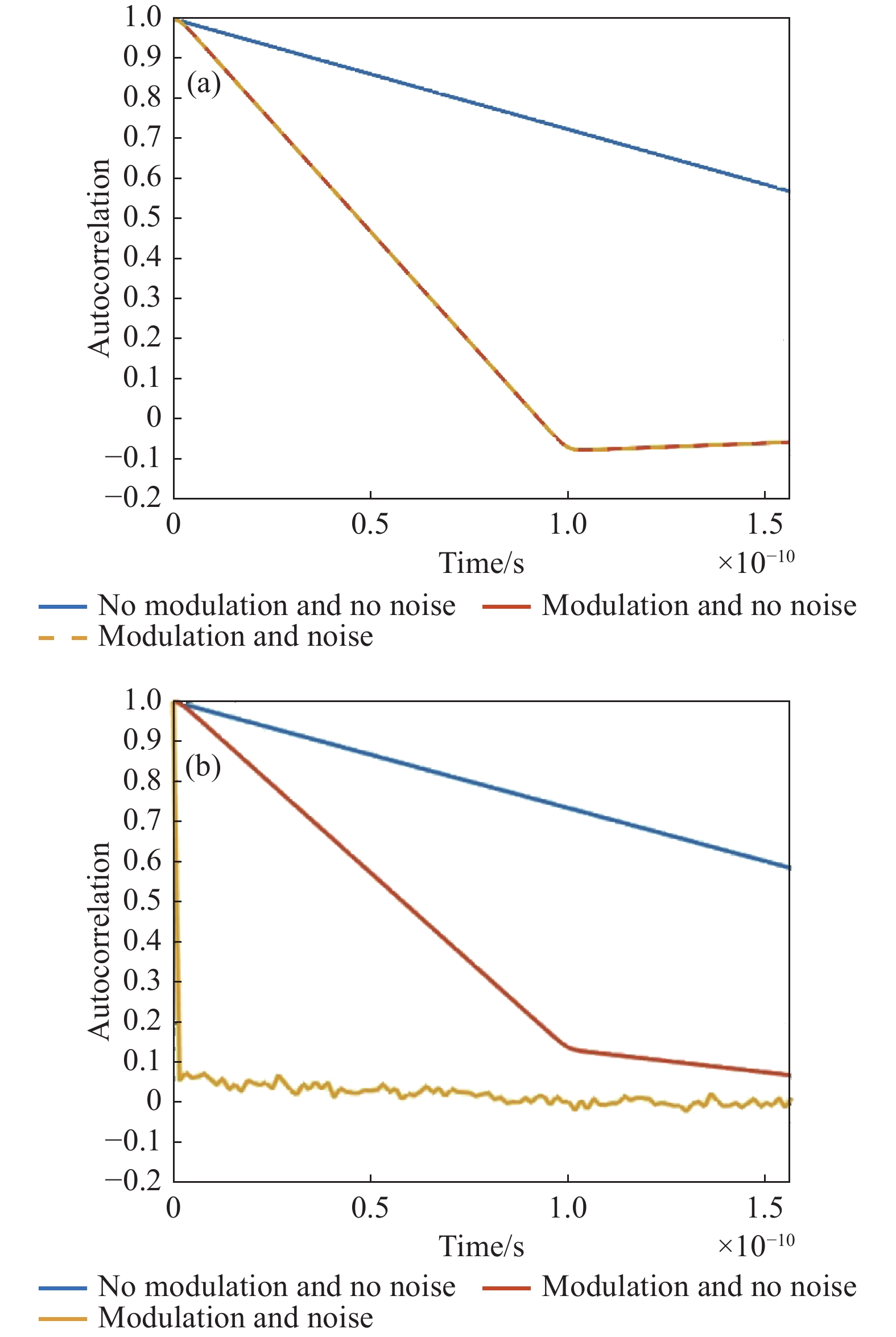
大气信道传输过程中,测量系统中有源器件的噪声会对光信号的功率产生影响。为了分析光信号传输过程中噪声对于光信道测量样本的自相关性的影响。针对单调制情况下,该小节分析了在其他参数固定,平均信噪比为12.01、−15.89 dB时,在无随机调制无噪声、有随机调制无噪声和有随机调制有噪声三种不同情况下,基于随机幅度调制的连续激光信号,在大气光信道中沿水平传输路径光信道测量样本去相关性,分析结果如图9(a)~(b)所示。需要说明的是,仿真过程中施加的噪声是加性噪声。仿真研究过程中平均信噪比主要通过调整信道衰减系数进行设置,平均信噪比为12.01、−15.89 dB的信道衰减系数分别为15、30 dB/km,传输距离为1 km。
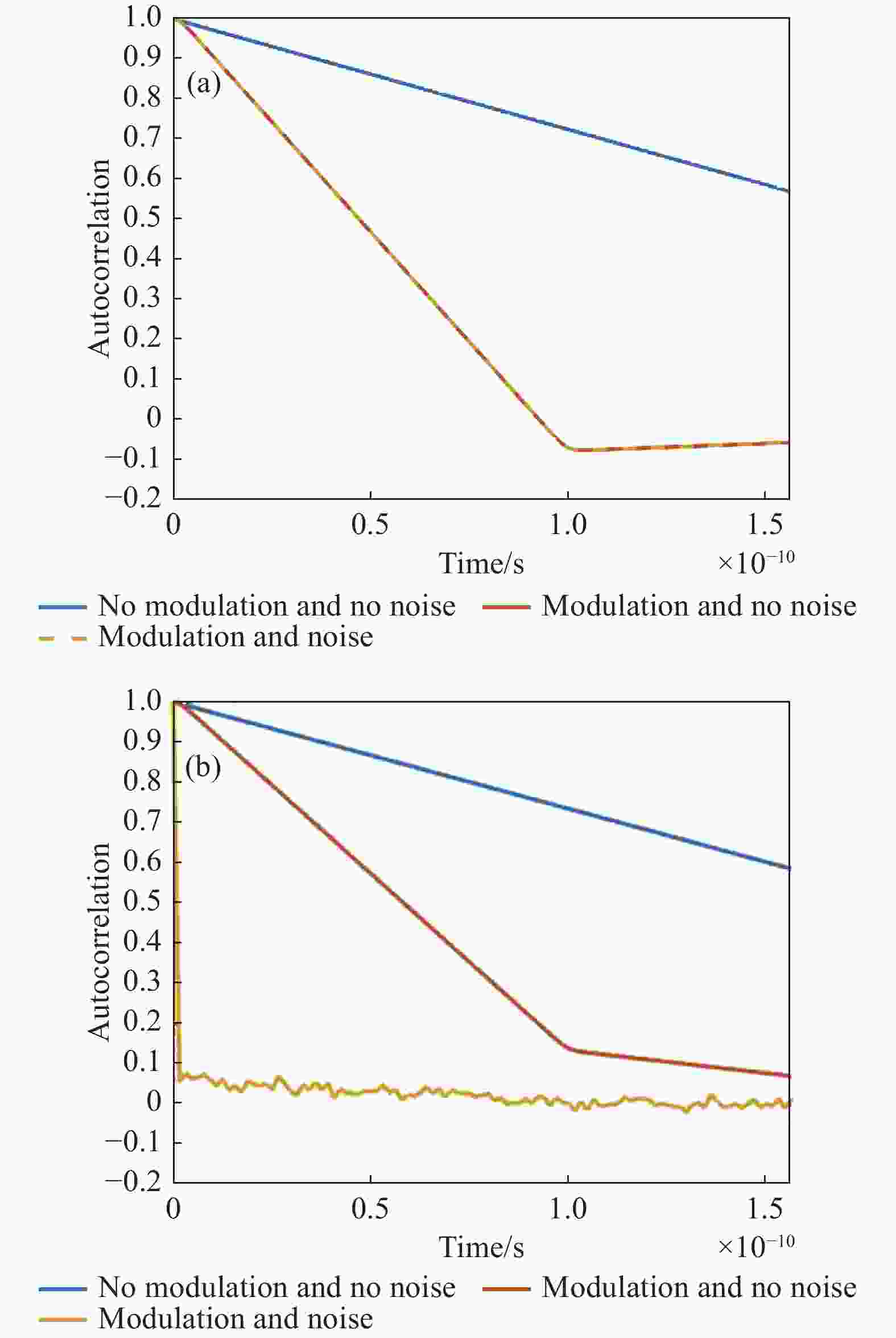
图 9 (a)信噪比为12.01 dB自相关对比分析图;(b)信噪比为 −15.89 dB自相关对比分析图
Figure 9. (a) Comparative analysis of autocorrelation with a SNR of 12.01 dB; (b) Comparative analysis of autocorrelation with a SNR of −15.89 dB
由图9(a)可知,在信噪比为12.01 dB(信号强度大于噪声强度)时,随着延迟时间的增加,对比有随机调制无噪声和有随机调制有噪声两种情况发现,黄色虚线和红线的变化趋势完全重合,说明噪声对于光信道测量样本的自相关性的影响相对较小。较高的信噪比可以减少噪声对测量结果的影响,提高信号分析的准确性。由图9(b)可知,在信噪比为−15.89 dB(信号强度小于噪声强度)时,加性噪声覆盖在光信号测量样本上,使得测量样本受到噪声的强烈干扰。对比有随机调制无噪声情况发现,有随机调制有噪声情况下测量样本的自相关特性变得模糊。
-
文中首先给出了基于随机调制实现光信道测量样本去相关的原理,并针对其实现测量样本去相关性进行了理论分析。利用OptiSystem软件搭建了基于随机调制的连续激光信号沿水平传输路径,在传输距离为1 km,大气折射率结构常数为$C_n^2 = 5 \times {10^{ - 15}}\;{\rm{{m}}^{ - 2/3}}$的大气光信道的测量样本去相关性仿真系统中,仿真过程中采用幅度调制。研究了无调制、单调制和双调制三种情况对于观测的光信道测量样本自相关性的影响。研究结果表明,对比无调制情况,在相同时间间隔内,观测到的光信道测量样本的测量数据变化次数增多;同时施加随机幅度调制的发射光信号,在小于湍流引起的光学波动的相关时间的采样间隔下,观测的光信道测量样本的自相关性降低。对单调制情形,得到不同大气光信道传输系数相干时间、伪随机码生成速率、传输距离和信噪比对于光信道测量样本自相关性的影响。当湍流强度、传输距离等参数一定条件下,随着大气光信道传输系数相干时间减小,延迟时间增加,测量样本的自相关性衰减速度更快,变化幅度更明显;随着伪随机码生成速率的加快,延迟时间的增加,测量样本的自相关性衰减速度更快,变化幅度更明显;当样本采样速率为$6.4 \times {10^6}$ Hz,伪随机码生成速率达到$6 \times {10^6}$ bit/s时,相邻测量样本的自相关性为0.112;当信噪比为12.01 dB时,噪声对于光信道测量样本的自相关性的影响相对较小。当信噪比为−15.89 dB时,随机调制实现光信道测量样本自相关特性变差。研究结果为大气光信道密钥生成产生具有优势的随机源提供了一定的理论依据。
Random modulation-based realization of optical channel measurement sample de-correlation analysis
-
摘要: 从大气光信道中可以提取两个合法通信方用来加密其传输的机密信息的公共密钥。首先,为了打破湍流引起的光学波动的相关时间对每秒提取的不相关光信道测量样本的数量限制,提出了为合法通信双方配备随机调制的方法,并针对其实现测量样本去相关性进行了理论分析;其次,利用OptiSystem软件仿真分析了大气光信道水平路径传输距离为1 km,中湍流,调制方式为幅度调制条件下,合法通信方在无调制、单调制、双调制三种不同调制的情况下对光信道测量样本自相关性的影响。针对单调制的情形,分析了不同大气光信道传输系数相干时间、伪随机码生成速率、传输距离和信噪比对光信道测量样本自相关性的影响。结果表明,对比无调制情况,在相同采样间隔内,观测到的光信道测量样本的测量数据变化次数增多;同时施加随机调制的发射光信号,在小于湍流引起的光学波动的相关时间的采样间隔下,观测到的光信道测量样本,在滞后100个样本的延迟时间后的自相关性,从无调制情况下的0.676降低到单调制情况下的0.083和双调制情况下的0.035。Abstract:
Objective Based on channel-based key extraction technology, the reciprocal random channel is treated as a public random source from which shared keys are generated. During the optical channel transmission, the received optical signals may exhibit correlation due to unstable factors such as atmospheric turbulence, indicating a degree of correlation between adjacent signal samples. In order to extract highly random key sources from the optical channel, it is necessary to reduce the measurement rate of the channel state based on the correlation time of the channel, ensuring the lack of correlation between consecutive channel measurements. To some extent, the correlation time of optical fluctuations caused by turbulence limits the number of uncorrelated optical channel measurement samples that can be obtained per second. Therefore, it is necessary to perform decorrelation on the continuous observed optical channel measurement samples obtained by the legitimate party at a sampling interval shorter than the correlation time of optical fluctuations caused by turbulence. In this paper, a simulation experiment based on random modulation is constructed to achieve decorrelation of measurement samples, and the impact of random modulation on the autocorrelation of measurement samples is analyzed. Methods Based on existing relevant theories, an experimental system for measuring sample decorrelation based on random modulation has been designed. The schematic diagram of the transmitting and receiving terminal principles based on random modulation is shown (Fig.1), and theoretical analysis has been conducted (Fig.2). Through analysis, the impact of the normalized variance of the modulation signal source on the correlation coefficient of consecutive measurements is explained. Utilizing OptiSystem software, a simulation experiment of the sample measurement system based on random modulation in optical channels was constructed (Fig.3). Results and Discussions The power samples of received signals over time were analyzed under three conditions of no modulation, single modulation, and double modulation (Fig.4). Moreover, the autocorrelation of measurement samples as a function of lag time was examined under different modulation conditions (Fig.5). In the absence of random modulation, it was observed that the autocorrelation after a lag of 100 samples is 0.676. Contrarily, under single modulation and double modulation conditions, the autocorrelation after a lag of 100 samples is 0.083 and 0.035, respectively. The utilization of random modulation effectively decreased the autocorrelation of optical channel measurement samples. Additionally, concerning the single modulation case, a separate analysis was conducted to assess the impact of varying the coherence time of the atmospheric optical channel transmission coefficient (Fig.6) and the effect of different pseudo-random code generation rates on the autocorrelation of optical channel measurement samples (Fig.7). When the sampling rate is 6.4 × 10⁶ Hz, and the generation rate is 6 × 106 bit/s, the autocorrelation of adjacent measurement samples is 0.112. This indicates that the use of random modulation enables obtaining nearly uncorrelated consecutive observations of optical channel measurement samples at a smaller sampling interval than the correlated time caused by turbulence-induced optical fluctuations. Finally, the impact of transmission distance (Fig.8) and signal-to-noise ratio (Fig.9) on the autocorrelation of measurement samples was analyzed. Conclusions The impact of three scenarios, namely no modulation, single modulation, and dual modulation, on the autocorrelation of the observed optical channel measurement samples was studied. The research results show that compared to the case without modulation, the number of measurement data variations in the observed optical channel measurement samples increases within the same time interval. Moreover, applying random amplitude modulation to the transmitted optical signal reduces the autocorrelation of the observed optical channel measurement samples at a sampling interval shorter than the correlation time of optical fluctuations caused by turbulence. When other parameters remain unchanged, as the coherence time of the atmospheric optical channel transmission coefficients decreases and the delay time increases, the autocorrelation of the measurement samples decays faster and the variation becomes more pronounced. Similarly, when other parameters remain unchanged, as the generation rate of pseudo-random codes increases and the delay time increases, the autocorrelation of the measurement samples decays faster. Additionally, the impact of increasing generation rate of pseudo-random codes on the autocorrelation of adjacent optical channel measurement samples was analyzed. -
Key words:
- laser communication /
- autocorrelation /
- random modulation /
- atmospheric turbulence
-
图 1 基于随机调制的收发端机原理示意图
Figure 1. Schematic diagram of the transceiver based on random modulation
图 2 (a)单调制情况下对${\tilde \phi _{{{\rm{A}}}}}\left( t \right)$两次连续观测值的相关系数分析图,$\sigma _{x,{{{\rm{A}}}}}^2 > 0,\sigma _{x,{{{\rm{B}}}}}^2 \equiv 0$;(b)双调制情况下对${\phi _{\rm{A}}}\left( t \right)$两次连续观测值的相关系数分析图,$\sigma _{x,{{{\rm{A}}}}}^2 \equiv \sigma _{x,{{{\rm{B}}}}}^2 > 0$
Figure 2. (a) Correlation coefficient analysis of two consecutive observations of ${\tilde \phi _{{{\rm{A}}}}}\left( t \right)$ in the case of signal modulation $\sigma _{x,{{{\rm{A}}}}}^2 > 0,\sigma _{x,{{{\rm{B}}}}}^2 \equiv 0$;(b) Correlation coefficient analysis of two consecutive observations of ${\phi _{{{\rm{A}}}}}\left( t \right)$ in the case of double modulation$\sigma _{x,{{{\rm{A}}}}}^2 \equiv \sigma _{x,{{{\rm{B}}}}}^2 > 0$
图 3 基于随机调制光信道样本测量系统示意图
Figure 3. Schematic diagram of optical channel sample measurement system based on random modulation
图 4 (a)无调制情况下实时测量数据图;(b)单调制情况下实时测量数据图;(c)双调制情况下实时测量数据图;(d)、(e)和(f)分别为不同调制情况下 0 ~ 0.119 × 10⁻³ s测量数据图
Figure 4. (a) Real-time measurement data plot in the case of no modulation; (b) Real-time measurement data plot in the case of single modulation; (c) Real-time measurement data plot in the case of double modulation; (d), (e), and (f) are the 0 -0.119 × 10⁻³ s measurement data plots in different modulation cases, respectively
图 5 不同调制情况下自相关性对比分析图
Figure 5. Comparative analysis of autocorrelation for different modulations
图 6 大气光信道传输系数不同相干时间对比分析图
Figure 6. Comparative analysis diagram of atmospheric optical channel transmission coefficients with different coherence times
图 7 (a) 伪随机码不同生成速率对比分析图;(b)相邻测量样本自相关分析图
Figure 7. (a) Comparative analysis diagram of pseudo random code with different generation rates; (b)Autocorrelation analysis diagram of adjacent measurement samples
图 8 不同距离情况下自相关性对比分析图
Figure 8. Plot of comparative analysis of autocorrelation at different distances
-
[1] 姜会林, 付强, 赵义武等. 空间信息网络与激光通信发展现状及趋势 [J]. 物联网学报, 2019, 3(2): 1-8. doi: 10.11959/j.issn.2096-3750.2019.00113 Jiang Huilin, Fu Qiang, Zhao Yiwu, et al. Development status and trend of space information network and laser communication [J]. Chinese Journal on Internet of Things, 2019, 3(2): 1-8. (in Chinese) doi: 10.11959/j.issn.2096-3750.2019.00113 [2] 王燕, 陈培永, 宋义伟, 等. 国外空间激光通信技术的发展现状与趋势 [J]. 飞控与探测, 2019, 2(1): 8-16. Wang Yan, Chen Peiyong, Song Yiwei, et al. Progress on the development and trend of overseas space laser communication technology [J]. Flight Control & Detection, 2019, 2(1):8-16. (in Chinese) [3] Kaushal H, Jain V K, Kar S. Free Space Optical Communication[M]. New Delhi: Springer (India), 2017. [4] Premnath S N, Jana S, Croft J, et al. Secret key extraction from wireless signal strength in real environments [J]. IEEE Transactions on Mobile Computing, 2012, 12(5): 917-930. [5] Wei Y, Kai Z, Mohapatra P. Adaptive wireless channel probing for shared key generation based on PID controller[J]. IEEE Transactions on Mobile Computing, 2013, 12(9): 1842-1852 . [6] Zeng K. Physical layer key generation in wireless networks: challenges and opportunities [J]. IEEE Communications Magazine, 2015, 53(6): 33-39. doi: 10.1109/MCOM.2015.7120014 [7] Chen C, Yang H. Shared secret key generation from signal fading in a turbulent optical wireless channel using common-transverse-spatial-mode coupling [J]. Optics Express, 2018, 26(13): 16422-16441 doi: 10.1364/OE.26.016422 [8] Bornman N, Forbes A, Kempf A. Random number generation and distribution out of thin (or thick) air [J]. Journal of Optics, 2020, 22(7): 075705. doi: 10.1088/2040-8986/ab9513 [9] Drake M D, Bas C F, Gervais D, et al. Optical key distribution system using atmospheric turbulence as the randomness generating function: classical optical protocol for information assurance [J]. Optical Engineering, 2013, 52(5): 055008. doi: 10.1117/1.OE.52.5.055008 [10] Banaszek K, Jachura M, Kolenderski P, et al. Optimization of intensity-modulation/direct-detection optical key distribution under passive eavesdropping [J]. Optics Express, 2021, 29(26): 43091-43103. doi: 10.1364/OE.444340 [11] Djordjevic I B. Atmospheric turbulence-controlled cryptosystems [J]. IEEE Photonics Journal, 2021, 13(1): 1-9. [12] Chen C, Jensen M A. Secret key establishment using temporally and spatially correlated wireless channel coefficients [J]. IEEE Transactions on Mobile Computing, 2010, 10(2): 205-215. [13] Li G, Hu A, Zhang J, et al. High-agreement uncorrelated secret key generation based on principal component analysis preprocessing [J]. IEEE Transactions on Communications, 2018, 66(7): 3022-3034. doi: 10.1109/TCOMM.2018.2814607 [14] Liu H, Wang Y, Yang J, et al. Fast and practical secret key extraction by exploiting channel response[C]//2013 Proceedings IEEE INFOCOM, 2013: 3048-3056. [15] Khisti A. Secret-key agreement over non-coherent block-fading channels with public discussion [J]. IEEE Transactions on Information Theory, 2016, 62(12): 7164-7178. doi: 10.1109/TIT.2016.2618861 [16] Chen D, Qin Z, Mao X, et al. SmokeGrenade: An efficient key generation protocol with artificial interference [J]. IEEE Transactions on Information Forensics and Security, 2013, 8(11): 1731-1745. doi: 10.1109/TIFS.2013.2278834 [17] Chen C, Li Q. Enhanced secret-key generation from atmospheric optical channels with the use of random modulation [J]. Optics Express, 2022, 30(25): 45862-45882. doi: 10.1364/OE.476856 [18] Yao H, Chen C, Ni X, et al. Analysis and evaluation of the performance between reciprocity and time delay in the atmospheric turbulence channel [J]. Optics Express, 2019, 27(18): 25000-25011. doi: 10.1364/OE.27.025000 [19] 吴健, 杨春平, 刘建斌. 大气中的光传输理论[M]. 北京:北京邮电大学出版社, 2005. -

 点击查看大图

计量
- 文章访问数: 34
- HTML全文浏览量: 11
- PDF下载量: 16
- 被引次数: 0

